2. Descent methods

2.1. Positioning the problem

Let \(K\) be the stiffness matrix (of size \(N\)) to be inverted, if it has the « good taste » of being symmetric definite positive (SPD in Anglo-Saxon literature), which is often [11] _ In the case of structural mechanics, it is shown by simple derivation that the following problems are equivalent:

• Resolution of the usual linear system with \(u\) solution vector (displacements or increments of movements, respectively in temperature…) and \(f\) vector translating the application of generalized forces to the thermo-mechanical system

\(({P}_{1})\text{Ku}=f\) (2.1-1)

• Minimization of the quadratic functional representing the energy of the system, with \(\text{< , >}\) the usual Euclidean dot product,

\(\begin{array}{}({P}_{2})u=\underset{v\in {\Re }^{N}}{\text{Arg}\text{min}}J(v)\\ \text{avec}J(v):=\frac{1}{2}\langle \text{v,Kv}\rangle -\langle f,v\rangle =\frac{1}{2}{v}^{T}\text{Kv}-{f}^{T}v\end{array}\) (2.1-2)

Because of the « definitive-positivity » of the matrix that makes \(J\) strictly convex, the cancelling vector [12] _ \(\nabla J\) corresponds to the unique [13] _ global minimum \(u\). This is illustrated by the following relationship, valid regardless of symmetric \(K\),

\(J(v)=J(u)+\frac{1}{2}{(v-u)}^{T}K(v-u)\) (2.1-3)

Thus, for any vector \(v\) different from the solution \(u\), the positive definite character of the operator makes the second term strictly positive and therefore \(u\) is also a global minimum.

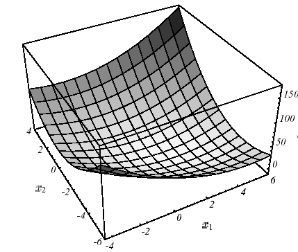
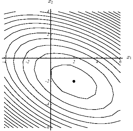
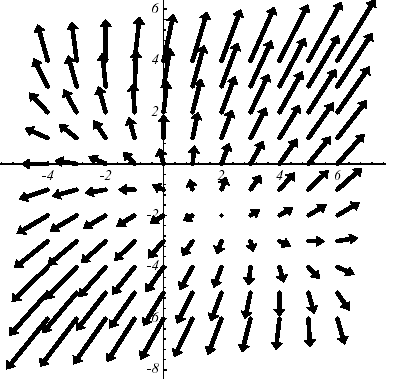
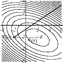
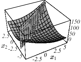
Figure 2.1-1. Example of \(J\) quadratic in \(N=2\) dimensions with \(K:=\left[\begin{array}{cc}3& 2\\ 2& 6\end{array}\right]\) and \(f:=\left[\begin{array}{c}2\\ -8\end{array}\right]\) : graph (a), level lines (b) and gradient vectors (c) .The spectrum of the operator is \(({\lambda }_{1};{v}_{1})=(7;{[\mathrm{1,2}]}^{T})\) and \(({\lambda }_{2};{v}_{2})=(2;{[-\mathrm{2,1}]}^{T})\) .

This very important result in practice is based entirely on this famous definition-positivity, a somewhat « ethereal » property of the work matrix. On a two-dimensional problem (\(N=2\)!) we can make a clear representation of it (cf. figure 2.1-1): the paraboloid form that focuses the single minimum at point \({[\mathrm{2,}-2]}^{T}\) with zero slope.

• Minimization of the energy norm of error \(e(v)=v-u\), which is more meaningful for mechanics,

\(\begin{array}{}({P}_{3})u=\underset{v\in {\Re }^{N}}{\text{Arg}\text{min}}E(v)\\ \text{avec}E(v):=\langle \text{Ke}(v),e(v)\rangle ={(\text{Ke}(v))}^{T}e(v)={\parallel e(v)\parallel }_{K}^{2}\end{array}\) (2.1-4)

From a mathematical point of view, it is nothing more than a matrix norm (legal since \(K\) is SPD). We often prefer to express it via a residue \(r(v)=f-\text{Kv}\)

\(E(v)=\langle r(v),{K}^{-1}r(v)\rangle =r{(v)}^{T}{K}^{-1}r(v)\) (2.1-5)

Notes:

• The scope of use of the conjugate gradient can in fact extend to any operator, not necessarily symmetric or definite positive or even square! To do this, we define the solution of ( \({P}_{1}\) ) as being that, in the sense of least squares, of the minimization problem

\(({P}_{2})\text{'}u=\underset{v\in {\Re }^{N}}{\text{Arg}\text{min}}{\parallel \text{Kv}-f\parallel }^{2}\) (2.1-6)

By derivation we arrive at so-called « normal » equations whose operator is square, symmetric and positive

\(({P}_{2})\text{''}\underset{\tilde{K}}{\underset{\underbrace{}}{{K}^{T}K}}u={K}^{T}f\) (2.1-7)

We can therefore apply a GC or a steepest-descent to it without too much hassle.

• The solution to the problem ( \({P}_{1}\) ) is at the intersection of \(N\) dimensional hyperplanes \(N-1\) . For example, for the case of Figure 2.1-1, it is expressed trivially in the form of intersections of lines:

\(\{\begin{array}{c}{\mathrm{3x}}_{1}+{\mathrm{2x}}_{2}=2\\ {\mathrm{2x}}_{1}+{\mathrm{6x}}_{2}=-8\end{array}\) (2.1-8)

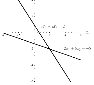
Figure 2.1-2. Solving example 1 by intersection of lines.

• Gradient methods differ from this philosophy, they are naturally part of the framework of minimizing a quadratic functional, in which they were developed and intuitively understood.

2.2. Steepest Descent

2.2.1. Principle

This last remark prefigures the philosophy of the so-called « steepest slope » method, better known under its Anglo-Saxon name of “Steepest Descent”: we build the series of iterates \({u}^{i}\) by following the direction in which \(J\) decreases the most, at least locally, that is to say \({d}^{i}=-\nabla {J}^{i}={r}^{i}\) with \({J}^{i}:=J({u}^{i})\text{et}{r}^{i}:=f-{\text{Ku}}^{i}\). At the i th iteration, we will therefore try to build \({u}^{i+1}\) such as:

\({u}^{i+1}:={u}^{i}+{\alpha }^{i}{r}^{i}\) (2.2-1)

and

\({J}^{i+1}<{J}^{i}\) (2.2-2)

Thanks to this formulation, we have therefore transformed a quadratic minimization problem of size \(N\) (in \(J\) and \(u\)) into a one-dimensional minimization (in \(G\) and \(\alpha\))

\(\begin{array}{}\text{Trouver}{\alpha }^{i}\text{tel que}{\alpha }^{i}=\underset{\alpha \in \left[{\alpha }_{m},{\alpha }_{M}\right]}{\text{Arg}\text{min}}{G}^{i}(\alpha )\\ \text{avec}{G}^{i}(\alpha ):=J({u}^{i}+\alpha {r}^{i})\end{array}\) (2.2-3)

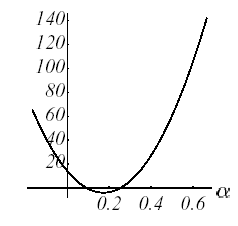
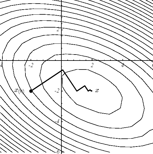
The following figures illustrate the operation of this procedure in example No. 1: starting from the point \({u}^{0}={[-\mathrm{2,}-2]}^{T}\) (cf. (a)), the optimal descent parameter, \({\alpha }^{0}\), is sought, along the line with the greatest slope \({r}^{0}\); this amounts to looking for a point belonging to the intersection of a vertical plane and a paraboloid (b), signified by the parabola (c). Trivially, this point cancels the derivative of the parabola (d).

\(\frac{\partial {G}^{0}({\alpha }^{0})}{\partial \alpha }=0\iff \langle \nabla J({u}^{1}),{r}^{0}\rangle =0\iff \langle {r}^{1},{r}^{0}\rangle =0\iff {\alpha }^{0}:=\frac{{\parallel {r}^{0}\parallel }^{2}}{\langle {r}^{0},{\text{Kr}}^{0}\rangle }\) (2.2-4)

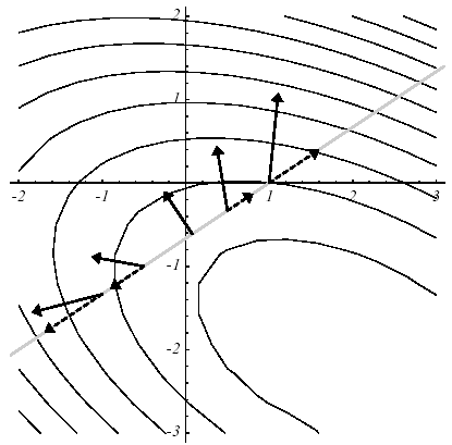
This orthogonality between two successive residues (i.e. successive gradients) produces a characteristic path, called a « zigzag » path, towards the solution (e). Thus, in the case of a poorly conditioned system producing narrow and elongated ellipses [14] _ , the number of iterations required can be considerable (cf. figure 2.2-1).

D

E

Figure 2.2-1. Illustration of the Steepest Descent on example 1: initial descent direction (a), intersection of surfaces (b), corresponding parabola (c), gradient vectors and their projection * along the initial descent direction (d) and overall process until convergence (e) .

2.2.2. Algorithm

Hence the unfolding

\(\begin{array}{}\text{Initialisation}{u}^{0}\text{donné}\\ \text{Boucle en}i\\ (1){r}^{i}=f-{\text{Ku}}^{i}(\text{nouveau résidu})\\ (2){\alpha }^{i}=\frac{{\parallel {r}^{i}\parallel }^{2}}{\langle {r}^{i},{\text{Kr}}^{i}\rangle }(\text{paramètre optimal de descente})\\ (3){u}^{i+1}={u}^{i}+{\alpha }^{i}{r}^{i}(\text{nouvel itéré})\\ (4)\text{Test d'arrêt via}{J}^{i+1}-{J}^{i}(\text{par exemple})\end{array}\)

Algorithm 1: Steepest Descent.

To save a matrix-vector product, it is preferable to replace step (1) by updating the following residue

\({r}^{i+1}={r}^{i}-{\alpha }^{i}{\text{Kr}}^{i}\) (2.2-5)

However, in order to avoid untimely accumulations of rounding, the residue is periodically recalculated with the initial formula (1).

2.2.3. Elements of theory

We show that this algorithm converges, for any starting point \({u}^{0}\), at the speed [15] _

\(\begin{array}{}{\parallel e({u}^{i+1})\parallel }_{K}^{2}={\omega }^{i}{\parallel e({u}^{i})\parallel }_{K}^{2}\\ \text{avec}{\omega }^{i}:=1-\frac{{\parallel {r}^{i}\parallel }^{4}}{\langle {K}^{-1}{r}^{i},{r}^{i}\rangle \langle {\text{Kr}}^{i},{r}^{i}\rangle }\end{array}\) (2.2-6)

By developing the error based on the \(({\lambda }_{j};{v}_{j})\) eigenmodes of the \(K\) matrix

\(e({u}^{i})={\sum }_{j}{\xi }_{j}{v}_{j}\) (2.2-7)

The energy error attenuation factor becomes

\({\omega }^{i}=1-\frac{{({\sum }_{j}{\xi }_{j}^{2}{\lambda }_{j}^{2})}^{2}}{({\sum }_{j}{\xi }_{j}^{2}{\lambda }_{j}^{3})({\sum }_{j}{\xi }_{j}^{2}{\lambda }_{j})}\) (2.2-8)

In (2.2-8), the fact that the \({\xi }_{j}\) components are squared ensures the priority avoidance of dominant eigenvalues. Here we find one of the characteristics of Krylov-type modal methods (Lanczos, Arnoldi cf. [Boi01] §5/§6) which favor extreme eigenmodes. For this reason, the Steepest Descent and the conjugate gradient are said to be « rough » compared to classical iterative solvers (Jacobi, Gauss-Seidel, SOR…) that are more « smooth » because they eliminate indiscriminately all the components at each iteration.

Finally, thanks to the Kantorovich inequality [16] _ , the readability of the attenuation factor is greatly improved. At the end of i iterations, at worst, the decrease is expressed in the form

\({\parallel e({u}^{i})\parallel }_{K}\le {(\frac{\eta (K)-1}{\eta (K)+1})}^{i}{\parallel e({u}^{0})\parallel }_{K}\) (2.2-9)

It ensures linear convergence [17] _

of the process in a number of iterations that is proportional to the conditioning of the operator. So, in order to get

\(\frac{{\parallel e({u}^{i})\parallel }_{K}}{{\parallel e({u}^{0})\parallel }_{K}}\le \varepsilon (\text{petit})\) (2.2-10)

You need a number of iterations in the order of

\(i\approx \frac{\eta (K)}{4}\text{ln}\frac{1}{\varepsilon }\) (2.2-11)

A poorly conditioned problem will therefore slow down the convergence of the process, which was already « visually » observed with the phenomenon of « narrow and tortuous valley ».

To better understand the involvement of the operator spectrum and the starting point in the development of the algorithm, let’s simplify the formula (2.2-8) by placing ourselves in the trivial case where \(N=2\). By noting \(\kappa =\frac{{\lambda }_{1}}{{\lambda }_{2}}\) the matrix conditioning of the operator and \(\mu =\frac{{\xi }_{2}}{{\xi }_{1}}\) the slope of the error at the i th iteration (in the coordinate system of the two eigenvectors), we obtain a more readable expression of the error attenuation factor (cf. figure 2.2-2)

\({\omega }^{i}=1-\frac{{({\kappa }^{2}+{\mu }^{2})}^{2}}{(\kappa +{\mu }^{2})({\kappa }^{3}+{\mu }^{2})}\) (2.2-12)

As for modal solvers, we note that the importance of operator conditioning is weighted by the choice of a good starting point: despite poor conditioning, cases (a) and (b) are very different; In the first, the starting point almost generates an operator’s own space and we converge in two iterations, otherwise they are the « eternal zigzags ».

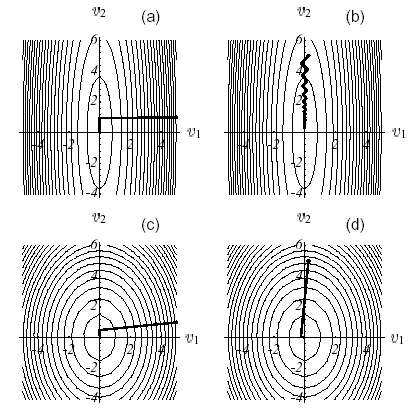
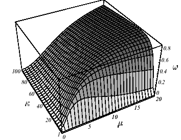
Figure 2.2-2. Convergence of the Steepest Descent on example 1 according to the values of the conditioning and the starting point: \(\kappa\) big and \(\mu\) small (a), \(\kappa\) and \(\mu\) big (b), \(\kappa\) and and \(\mu\) small (c), small (c), \(\kappa\) small (c), small (c), small and \(\mu\) big (d) and overall shape of \(\omega =\omega (\kappa ,\mu )\) (e) .

Notes:

This steepest method was initiated by Cauchy (1847) and brought up to date by Curry (1944). In the context of SPD operators, it is also sometimes called the optimal parameter gradient method (cf. [:ref:`LT98 <LT98>`] §8.2.1). Despite its weak convergence properties, it has had its « heyday » for minimizing almost any :math:`J`*functions, in fact only derivable. In this more general case, it then only makes it possible to reach stationary points, at best local minima.

• To avoid zig-zag effects, various acceleration methods have been proposed (cf.Forsythe 1968, Luenberger 1973 or [Min08] §2.3) which have a convergence speed similar to that of the conjugate gradient but for a much greater computational complexity. So they gradually fell into disuse.

• Note that variants of algorithm 1 have been introduced to deal with cases not SPD: Iteration of the minimum residue and Steepest Descent with residue standard (cf. [Saa03]).

• Through Steepest Descent, we find a key concept that is very common in numerical analysis: that of solving a problem, by projecting iterates onto an approximate subspace, here \({K}_{i}:=\mathrm{vect}({r}^{i})\) , perpendicular to another subspace, here \({L}_{i}:={K}_{i}\). They are called, respectively, search or approximation space and constraint space. For the Steepest Descent, they are equal and reduced to their simplest expression but we will see that for the conjugate gradient they take the form of particular spaces, called Krylov spaces.

Formally, at each iteration \(i\) of the algorithm, we thus look for an increment \({\delta }^{i}:={\alpha }^{i}{r}^{i}\) such that:

\(\{\begin{array}{c}{u}^{i}:={u}^{0}+{\delta }^{i}{\delta }^{i}:={\alpha }^{i}{r}^{i}\in {K}_{i}\\ \langle {r}^{0}-K{\delta }^{i},w\rangle =0\forall w\in {L}_{i}={K}_{i}\end{array}\) (2.2-13)

This general framework is what we call Petrov-Galerkin conditions.

2.2.4. Complexity and memory occupancy

Most of the calculation cost of algorithm 1 lies in the update (2.2-5) and, more particularly, in the matrix-vector product \(K{r}^{i}\). On the other hand, it has already been mentioned that its convergence was acquired and took place in a number of iterations proportional to the conditioning of the matrix (cf. (2.2-11)).

The computational complexity of the algorithm is therefore, if we take into account the empty nature of the operator, is of the order of \(\Theta (\eta (K)\text{cN})\) where \(c\) is the average number of non-zero terms per line of \(K\).

Thus, with problems resulting from finite element discretization of second-order elliptic operators [18] _ (resp. of the fourth order), we have operator packages in \(\eta (K)=\Theta ({N}^{2/d})\) (resp. \(\eta (K)=\Theta ({N}^{4/d})\)) where \(d\) the space dimension. The computational complexity of the Steepest Descent in this framework is written as \(\Theta ({\text{cN}}^{\frac{2}{d}+1})\) (resp. \(\Theta ({\text{cN}}^{\frac{4}{d}+1})\)).

In terms of memory occupancy, only the storage of the working matrix is possibly required [19] _ : \(\Theta (\text{cN})\). In practice, the computer implementation of sparse storage requires the management of additional integer vectors: for example, for the MORSE storage used in Code_Aster, vectors of the end-of-line indices and column indices of the non-zero elements of the profile. Hence an effective memory complexity of \(\Theta (\text{cN})\) real and \(\Theta (\text{cN}+N)\) integers.

2.3. « General » descent method

2.3.1. Principle

A crucial step in these methods is choosing their direction of descent [20] _ . Even if the functional gradient remains the main ingredient, we can definitely choose another \({d}^{i}\) version than the one required for the Steepest Descent. At the i th iteration, we will therefore try to build \({u}^{i+1}\) verifying

\({u}^{i+1}:={u}^{i}+{\alpha }^{i}{d}^{i}\) (2.3-1)

with

\({\alpha }^{i}=\underset{\alpha \in \left[{\alpha }_{m},{\alpha }_{M}\right]}{\text{Arg}\text{min}}J({u}^{i}+\alpha {d}^{i})\) (2.3-2)

This is of course only a generalization of the “Steepest Descent” seen previously and it is shown that its choices of the descent parameter and its orthogonality property are generalized.

\(\begin{array}{}{\alpha }^{i}:=\frac{\langle {r}^{i},{d}^{i}\rangle }{\langle {d}^{i},{\text{Kd}}^{i}\rangle }\\ \langle {d}^{i},{r}^{i+1}\rangle =0\end{array}\) (2.3-3)

Hence the same « zigzag » effect during the process and a convergence similar to (2.2-6) with an error attenuation factor reduced by:

\({\omega }^{i}:=1-\frac{{\langle {r}^{i},{d}^{i}\rangle }^{2}}{\langle {K}^{-1}{r}^{i},{r}^{i}\rangle \langle {\text{Kd}}^{i},{d}^{i}\rangle }\ge \frac{1}{\eta (K)}{\langle \frac{{r}^{i}}{\parallel {r}^{i}\parallel },\frac{{d}^{i}}{\parallel {d}^{i}\parallel }\rangle }^{2}\) (2.3-4)

From this result we can then formulate two observations:

• The conditioning of the operator intervenes directly on the attenuation factor and therefore on the speed of convergence,

• To ensure convergence (sufficient condition), during a given iteration, the direction of descent must not be orthogonal to the residue.

The sufficient condition of this last item is of course verified for the Steepest Descent (\({d}^{i}={r}^{i}\)) and it will impose a choice of descent direction for the conjugate gradient. To overcome the problem raised by the first point, we will see that it is possible to constitute a \(\tilde{K}\) worker whose packaging is less extensive. We then speak of preconditioning.

Still in the case of an operator SPD, the flow of a « general » descent method is therefore written as

\(\begin{array}{}\text{Initialisation}{u}^{0},{d}^{0}\text{donnés,}{r}^{0}=f-{\text{Ku}}^{0}\\ \text{Boucle en}i\\ (1){z}^{i}={\text{Kd}}^{i}\\ (2){\alpha }^{i}=\frac{\langle {r}^{i},{d}^{i}\rangle }{\langle {d}^{i},{z}^{i}\rangle }(\text{paramètre optimal de descente})\\ (3){u}^{i+1}={u}^{i}+{\alpha }^{i}{d}^{i}(\text{nouvel itéré})\\ (4){r}^{i+1}={r}^{i}-{\alpha }^{i}{z}^{i}(\text{nouvel résidu})\\ (5)\text{Test d'arrêt via}{J}^{i+1}-{J}^{i},\parallel {d}^{i}\parallel \text{ou}\parallel {r}^{i+1}\parallel (\text{par exemple})\\ (6)\text{Calcul de la dd}{d}^{i+1}={d}^{i+1}(\nabla {J}^{k},{\nabla }^{2}{J}^{k},{d}^{k}\dots )\end{array}\)

Algorithm 2: Descent method in the case of a quadratic functional.

This algorithm already prefigures the Conjugate Gradient (GC) algorithm that we will examine in the next chapter (cf. algorithm 4). It clearly shows that GC is only a descent method applied within the framework of quadratic functions and specific descent directions. Finally, only step (6) will be expanded.

Notes:

• By successively setting the canonical vectors of the coordinate axes of space at \(N\) dimensions ( \({d}^{i}={e}_{i}\) ) as directions of descent, we obtain the Gauss-Seidel method.

• To avoid the additional cost of calculating the one-dimensional minimization step (2) (matrix-vector product), one can choose to set the descent parameter arbitrarily: it is the Richardson method that converges at best, like the Steepest Descent.

2.3.2. Complements

With any continuous \(J\) function (cf. figure 2.3-1), we go beyond the strict framework of linear system inversion for that of nonlinear continuous optimization without constraints (\(J\) is then often called cost function or objective function). Two simplifications that had existed hitherto become illegal then become illegal:

• Updating the residue: step (4),

• Simplified calculation of the optimal descent parameter: step (2).

Their raison d’être being only to use all the hypotheses of the problem to facilitate one-dimensional minimization (2.3-2), one is then forced to explicitly perform this linear search on a more chaotic functional with this time multiple local minima. Fortunately, there are a variety of methods depending on the level of information required on the cost function \(J\):

• \(J\) (quadratic interpolation, dichotomy on the values of the function, the golden section, Goldstein and Price rule…),

• \(J,\nabla J\) (dichotomy on the values of the derivative, Wolfe rule, Armijo rule…),

• (\(J,\nabla J,{\nabla }^{2}J\) Newton-Raphson…)

*…

As far as the direction of descent is concerned, again, numerous solutions are proposed in the literature (conjugated nonlinear gradient, Quasi-Newton, Newton, Levenberg-Marquardt [21] _ …). For a long time, the so-called nonlinear conjugate gradient methods (Fletcher-Reeves (FR) 1964 and Polak-Ribière (PR) 1971) have proved to be interesting: they converge superlinearly towards a local minimum for reduced calculation costs and reduced memory space (cf. Figures 2.3-1).

They lead to the choice of an additional parameter \({\beta }^{i}\) which manages the linear combination between the descent directions

\({d}^{i+1}=-\nabla {J}^{i+1}+{\beta }^{i+1}{d}^{i}\text{avec}{\beta }^{i+1}:=\{\begin{array}{c}\frac{{\parallel \nabla {J}^{i+1}\parallel }^{2}}{{\parallel \nabla {J}^{i}\parallel }^{2}}(\text{FR})\\ \frac{\langle \nabla {J}^{i+1},\nabla {J}^{i+1}-\nabla {J}^{i}\rangle }{{\parallel \nabla {J}^{i}\parallel }^{2}}(\text{PR})\end{array}\) (2.3-5)

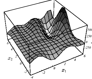
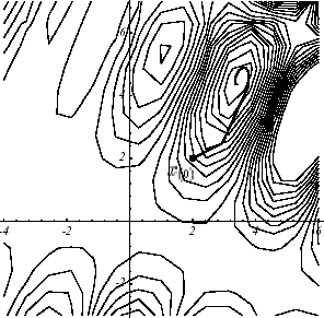
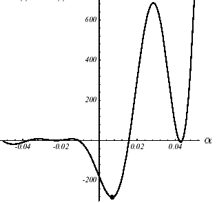
Figure 2.3-1. Example of \(J\) non-convex in \(N=2\) : graph (a): graph (a), convergence with a non-linear GC of the Fletcher-Reeves type (b), section plan * of the first one-dimensional search (c) .

Hence the algorithm, by naming \({r}^{0}\) the opposite of the gradient and no longer the residue (which no longer needs to be here),

\(\begin{array}{}\text{Initialisation}{u}^{0}\text{donné,}{r}^{0}=-\nabla {J}^{0},{d}^{0}={r}^{0}\\ \text{Boucle en}i\\ (1)\text{Trouver}{\alpha }^{i}=\underset{\alpha \in \left[{\alpha }_{m},{\alpha }_{M}\right]}{\text{Arg}\text{min}}J({u}^{i}+\alpha {d}^{i})(\text{paramètre de descente})\\ (2){u}^{i+1}={u}^{i}+{\alpha }^{i}{d}^{i}(\text{nouvel itéré})\\ (3){r}^{i+1}=-\nabla {J}^{i+1}(\text{nouveau gradient})\\ (4)\text{Test d'arrêt via}{J}^{i+1}-{J}^{i},\parallel {d}^{i}\parallel \text{ou}\parallel {r}^{i+1}\parallel (\text{par exemple})\\ (5){\beta }^{i+1}=\{\begin{array}{c}\frac{{\parallel {r}^{i+1}\parallel }^{2}}{{\parallel {r}^{i}\parallel }^{2}}(\text{FR})\\ \frac{\langle {r}^{i+1},{r}^{i+1}-{r}^{i}\rangle }{{\parallel {r}^{i}\parallel }^{2}}(\text{PR})\end{array}(\text{paramètre de conjugaison})\\ (6){d}^{i+1}={r}^{i+1}+{\beta }^{i+1}{d}^{i}(\text{nouvelle dd})\end{array}\)

Algorithm 3: Nonlinear conjugate gradient methods (FR and PR) .

The term conjugate nonlinear gradient is instead synonymous with « non-convex » here: there is no longer a dependency between the minimization problem (\({P}_{2}\)) and a linear system (\({P}_{1}\)). In view of algorithm 4, the major similarities with the GC therefore seem quite clear. In the context of a quadratic cost function of the type (2.1-2b), all that is needed is to replace step (1) with updating the residue and calculating the optimal descent parameter. GC is only a Fletcher-Reeves method applied to the case of a convex quadratic functional.

Now that we have successfully started the link between the descent methods, the conjugate gradient in the sense of linear solver SPD and its version, seen from the end of the telescope nonlinear continuous optimization, we will (finally!) get to the heart of the matter and argue for the choice of a descent direction of the type (2.3-5) for the standard GC. For more information on descent-type methods, the reader may refer to the excellent optimization books (in French) by M. Minoux [Min08], J.C. Culioli [Cu94] or J.F.Bonnans et al. [BGLS].

[1]

For a simulation via Code_Aster, the matrix is often undefined due to the addition of additional variables (called « de Lagranges ») to impose limit conditions [Pel01].

[2]

Derivative cancellation is a particular case of the convex and unconstrained case of the famous Kuhn-Tucker relationships characterizing the optimum of a differentiable optimization problem. It is called the « Euler equation. »

[3]

Without this convexity, we are not assured of uniqueness. It is then necessary to deal with local minima!

[4]

The conditioning of the \(K\) operator is written as the ratio of its extreme eigenvalues \(\eta (K):=\frac{{\lambda }_{\text{max}}}{{\lambda }_{\text{min}}}\) which are themselves proportional to the axes of the ellipses. Hence a direct and visual link between poor matrix conditioning and a narrow and tortuous valley where minimization is abused.

[5]

The positivity definition of the operator assures us of the « good nature » of the \({\omega }^{i}\) parameter. It is indeed a mitigating factor because \(0\le {\omega }^{i}\le 1\).

[6]

Whatever \(K\) matrix SPD and \(u\) non-zero vector: \(1\le \frac{\langle \text{Ku},u\rangle \langle {K}^{-1}u,u\rangle }{{\parallel u\parallel }_{2}^{4}}\le \frac{{(\eta {(K)}^{}+\eta {(K)}^{})}^{2}}{4}\)).

[7]

That is \(\underset{i\to \infty }{\text{lim}}\frac{J({u}^{i+1})-J(u)}{J({u}^{i})-J(u)}\le \alpha :={(\frac{\eta (K)-1}{\eta (K)+1})}^{2}<1\). The asymptotic convergence rate \(\alpha\) is called the Kantorovich ratio

[8]

Case most often encountered in structural mechanics.

[9]

In absolute terms, the Steepest Descent like the GC only requires knowledge of the action of the matrix on any vector and not its extensive storage. This facility can be valuable for applications that require very many degrees of freedom (CFD).

[10]

By definition a direction of descent (dd) at the th stage, noted \({d}^{i}\), verifies: \({(\nabla {J}^{i})}^{T}{d}^{i}<0\).

[11]

These last two methods are used by Code_Aster: the first in the nonlinear operators (STAT/DYNA/THER_NON_LINE), the second in the realignment macro (MACR_RECAL).