4. The Preconditioned Conjugate Gradient (GCPC)#
4.1. General description#
4.1.1. Principle#
As we have seen (and hammered!) in the preceding paragraphs, the speed of convergence of the descent methods, and in particular that of the conjugate gradient, depends on the conditioning of the matrix \(\eta (K)\). The closer it is to its floor value, 1, the better the convergence.
The preconditioning principle is then « simple », it consists in replacing the linear system of the problem (\({P}_{1}\)) by an equivalent system of the type (preconditioning on the left):
\(({\tilde{P}}_{1})\underset{\tilde{K}}{\underset{\underbrace{}}{{M}^{-1}K}}u=\underset{\tilde{f}}{\underset{\underbrace{}}{{M}^{-1}f}}\) (4.1-1)
such as, ideally:
The conditioning is obviously improved (this theoretical property, like the following, are only very rarely demonstrated. They are often only supported by digital experiences): :math:`eta (tilde{K})ll eta (K)` . *
Just like the spectral distribution: smaller eigenvalues.
\({M}^{-1}\) is inexpensive to evaluate (as for the initial operator, we often just need to know the action of the preconditioner on a vector): \(\text{Mv}=u\) easy to reverse.
Even easy to implement and, possibly, effective to parallelize.
That it be as hollow as the initial matrix because it is a question of limiting additional memory congestion.
That it keeps the same properties as the initial one in the work matrix \(\tilde{K}\): here, the character SPD.
In theory, the best choice would be \({M}^{-1}={K}^{-1}\) because then \(\eta (\tilde{K}={I}_{N})=1\), but if you have to completely reverse the operator by a direct method to build this preconditioner, it is of little practical interest! However, we will see later that this idea is not as far-fetched as that.
In other words, the objective of a preconditioner is to narrow the spectrum of the work operator so, as already mentioned, his « effective conditioning » will be improved along with the convergence of GCPC.
Graphically, this results in a more spherical shape of the graph than the quadratic form. Even on a \(N=2\) dimensional system and with a « crude » preconditioner (cf. figure 4.1-1), the effects are significant.
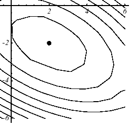
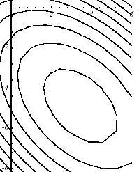
Figure 4.1-1. Effect of diagonal preconditioning on the paraboloid of example 1: (a) without, \(\eta (K)=3.5\) , (b) with, \(\eta (\tilde{K})=2.8\) .
In absolute terms, you can precondition a linear system from the left (“left preconditioning”), from the right (resp. “right”) or by doing a mixture of the two (resp. “split”). It is this last version that will be retained for our operator SPD, because we cannot directly apply the GC to solve \(({\tilde{P}}_{1})\): even if \({M}^{-1}\) and \(K\) are SPD, this is not necessarily the case for their product.
The trick then consists in using a preconditioning matrix SPD, \(M\), for which we will therefore be able to define another matrix (\(M\) being real symmetric, it can be diagonalized in the form \(M\mathrm{=}{\text{UDU}}^{T}\) with \(D\mathrm{:}\mathrm{=}\text{diag}({\lambda }_{i}){\lambda }_{i}>0\) and \(U\) orthogonal matrix). The matrix SPD sought then comes from the associated decomposition \({M}^{1\mathrm{/}2}\mathrm{=}\text{Udiag}(\sqrt{{\lambda }_{i}}){U}^{T}\) with \({M}^{1/2}\) defined as \({({M}^{1/2})}^{2}=M\). Hence the new work problem, this time SPD
\(({\stackrel{ˆ}{P}}_{1})\underset{\stackrel{ˆ}{\mathrm{K}}}{\underset{\underbrace{}}{{\mathrm{M}}^{\mathrm{-}1\mathrm{/}2}{\text{KM}}^{\mathrm{-}1\mathrm{/}2}}}\underset{\stackrel{ˆ}{\mathrm{u}}}{\underset{\underbrace{}}{{\mathrm{M}}^{1\mathrm{/}2}\mathrm{u}}}\mathrm{=}\underset{\stackrel{ˆ}{\mathrm{f}}}{\underset{\underbrace{}}{{\mathrm{M}}^{\mathrm{-}1\mathrm{/}2}\mathrm{f}}}\) (4.1-2)
on which we will be able to apply the standard GC algorithm to constitute what is called a Preconditioned Conjugate Gradient (GCPC).
4.1.2. Algorithm#
In short, by substituting in algorithm 4, the expressions from the previous problem \(({\stackrel{ˆ}{P}}_{1})\) and by working a bit on simplifying everything to only manipulate expressions in \(K\), \(u\) and \(f\), the following procedure occurs.
\(\begin{array}{}\text{Initialisation}{u}^{0}\text{donné,}{r}^{0}={\text{f-Ku}}^{0},{d}^{0}={M}^{-1}{r}^{0},{g}^{0}={d}^{0}\\ \text{Boucle en}i\\ (1){z}^{i}={\text{Kd}}^{i}\\ (2){\alpha }^{i}=\frac{\langle {r}^{i},{g}^{i}\rangle }{\langle {d}^{i},{z}^{i}\rangle }(\text{paramètre optimal de descente})\\ (3){u}^{i+1}={u}^{i}+{\alpha }^{i}{d}^{i}(\text{nouvel itéré})\\ (4){r}^{i+1}={r}^{i}-{\alpha }^{i}{z}^{i}(\text{nouveau résidu})\\ (5)\text{Test d'arrêt via}\langle {r}^{i+1},{r}^{i+1}\rangle (\text{par exemple})\\ (6){g}^{i+1}={M}^{-1}{r}^{i+1}(r\text{ésidu préconditionné})\\ (7){\beta }^{i+1}=\frac{\langle {r}^{i+1},{g}^{i+1}\rangle }{\langle {r}^{i},{g}^{i}\rangle }(\text{paramètre de conjugaison optimal})\\ (8){d}^{i+1}={g}^{i+1}+{\beta }^{i+1}{d}^{i}(\text{nouvelle dd})\end{array}\)
Algorithm 5: Preconditioned conjugate gradient (GCPC) .
But in fact, the symmetric nature of the initial preconditioned problem \(({\tilde{P}}_{1})\) is all relative. It is inseparable from the underlying dot product. If instead of taking the usual Euclidean dot product, we use a matrix dot product defined with respect to \(K\), \(M\) or \({M}^{-1}\), it is possible to symmetrize the preconditioned problem that was not initially preconditioned. As with Krylov’s methods in modal, it is the couple (work operator, scalar product) that must be modulated to adapt to the problem!
Thus, \({M}^{-1}K\) being symmetric with respect to the \(M\) -dot product, we can substitute this new work operator and this new dot product in the non-preconditioned GC algorithm (algorithm 4)
\(\begin{array}{}K\Leftarrow {M}^{-1}K\\ \langle ,\rangle \Leftarrow {\langle ,\rangle }_{M}\end{array}\)
And (O surprise!) by working the expressions a bit, we find exactly the algorithm of the previous GCPC (algorithm 5). We proceed in the same way with preconditioning on the right, \(K{M}^{-1}\), via a \({M}^{-1}\) -scalar product. So preconditioning to the right, to the left, or « splitted in fashion SPD », all lead rigorously to the same algorithm. This observation will be useful to us later when we realize that the matrices provided by*Code_Aster* (and also the preconditioners that we will associate with them) do not always conform to the ideal scenario \(({\stackrel{ˆ}{P}}_{1})\).
Notes:
This variant of GCPC, which is by far the most common, is sometimes referred to in the literature as: “untransformed preconditioned conjugate gradient”. As opposed to the transformed version that manipulates the specific entities of the new formulation.
General descent methods and, especially non-linear GCs, are also preconditioned (cf. [§2.3]). This time with a preconditioner approximating the inverse of the Hessian at the point in question, so as to make the graph of the functional in the vicinity of this point spherical.
4.1.3. « Overview » of the main preconditioners#
The solution, often chosen for its simplicity of implementation, its « numerical efficiency/additional calculation cost » ratio for problems that are not too poorly conditioned, consists in preconditioning the initial operator by using the diagonal.
\({M}_{J}:=\text{diag}({K}_{\text{ii}})\) (4.1-3)
This is called diagonal or Jacobi preconditioning (JCG for “Jacobi Conjugate Gradient”) in reference to the stationary method of the same name.
Notes:
This is a solution often chosen in CFD (for EDF R&D: Code_Saturne, TELEMAC). In these areas, a great deal of attention to the nonlinear resolution scheme and to the construction of the mesh produces a problem that is often better conditioned. This is what made the JCG famous, transformed for the occasion into a real « racing horse » dedicated to large parallel computers.
It is a solution proposed, in structural mechanics, by a good number of commercial codes: ANSYS, Zebulon, NASTRAN. It was present in Code_Aster but its lack of reliability led to its resorption.
This principle of preconditioning « of the poor » extends to methods of descent, this time taking the Hessian diagonal.
Another very common preconditioner is SSOR (for Symetric Successive Over Relaxation). Like the previous one, it is deduced from a classical iterative method: the relaxed Gauss-Seidel method. By decomposing the initial operator into the usual form \(K:=D+L+{L}^{T}\) where \(D\) is its diagonal and \(L\) is its strictly lower triangular part, it is written (according to the relaxation parameter \(\omega\))
\({M}_{\text{SSOR}}(\omega ):=\frac{1}{\omega (\omega -2)}(D+\mathrm{\omega L}){D}^{-1}(D+{\mathrm{\omega L}}^{T})0<\omega <2\) (4.1-4)
It has the advantage of not requiring memory storage and additional calculation costs, since it is directly developed from \(K\), while being very simple to reverse (a descent-ascent). On model problems (the famous « Laplacian on the unit square »), theoretical results have been unearthed in finite elements.
\(\eta (K):=\Theta (\frac{1}{{h}^{2}})\Rightarrow \eta ({M}^{-1}K):=\Theta (\frac{1}{h})\) (4.1-5)
On the other hand, it has the option, for an operator SPD, to limit its spectrum in the \(]\mathrm{0,1}]\) band. However, it has proven in industrial practice to be less effective than the incomplete Cholesky preconditioners that we will discuss in the next paragraph. And it poses the delicate problem of choosing the optimal relaxation parameter, which is by nature very « problem-dependent ».
Notes:
This preconditioner was proposed by D.J.Evans (1967) and studied by O.Axelsson (1974). It is available in many versions: non-symmetric, in blocks, with optimal relaxation parameter…
By asking \(\omega =1\) we find the particular case of Gauss-Seidel Symmetric
\({M}_{\text{SGS}}(\omega ):=-(D+L){D}^{-1}(D+{L}^{T})\) (4.1-6)
A host of other preconditioners have thus emerged over the past thirty years in the literature: explicit (polynomials [BH89], SPAI, AINV…), implicit (Schwarz, IC…), multilevels (domain decomposition, multigrids…)… Some are specific to an application, others more general. The « fashion effects » have also done their job! For more information you can consult the monumental sum committed by G.Meurant [Meu99] or the books by Y.Saad [Saa03] and H.A.Van der Vorst [Van01].
4.2. Incomplete Cholesky factorization#
4.2.1. Principle#
We have just seen that preconditioners are often inspired by fully-fledged linear solvers: Jacobi for the diagonal one, Gauss-Seidel for SSOR. The one based on an Incomplete Cholesky factorization (IC) is no exception to the rule! But this time it relies not on another iterative method, but on a direct method such as Cholesky. Hence the name ICCG (“Incomplete Cholesky Conjugate Gradient”) given to the coupling of this preconditioner with GCPC.
The initial operator being SPD, it admits a Cholesky decomposition of the \(K={\mathrm{CC}}^{T}\) type where \(C\) is a lower triangular matrix. We call incomplete Cholesky factorization, the search for a lower triangular \(F\) matrix that is as sparse as possible and such that \({\mathrm{FF}}^{T}\) is close to \(K\) in a sense to be defined. For example, by asking \(B=K-{\mathrm{FF}}^{T}\) we will ask that the relative error (expressed in a matrix norm of your choice)
\(\Delta :=\frac{\parallel B\parallel }{\parallel K\parallel }\) (4.2-1)
be as small as possible. Reading this « fairly evasive » definition, one glimpses the profusion of possible scenarios. Everyone went at it with their own incomplete factorization! The book by G.Meurant [Meu99] shows the great diversity: \(\mathrm{IC}(n)\), \(\mathrm{MIC}(n)\), relaxed, reordered, in blocks…
However, to simplify the task, we often impose a priori the sparse structure of \(F\), that is to say its graph
\(\Theta (F):=\left\{(i,j),1\le j\le i-\mathrm{1,}1\le i\le N,{F}_{\text{ij}}\ne 0\right\}\) (4.2-2)
It is obviously a question of finding a compromise: the more this graph is extended and the smaller the error (4.2-1) will be, but the more expensive will be the calculation and storage of what is (in the case in which we are interested) only a preconditioner. Generally, preconditioners are recursive and at their basic level, they impose on \(F\) the same structure as that of \(C\): \(\Theta (F)=\Theta (C)\).
Notes:
Initially, these incomplete factorizations were developed to iteratively solve a linear system of type (\({P}_{1}\))
\({\text{FF}}^{T}{u}^{i+1}\mathrm{=}f\mathrm{-}{\text{Bu}}^{i}\) (4.2-3)
The « nerve of war » then being the spectral ray \(\rho \left[{({\text{FF}}^{T})}^{\mathrm{-}1}B\right]\) * that a careful choice of \(\Theta (F)\) can contribute significantly to reducing.
This principle of incomplete factorization is easily generalized to the standard case where the operator is written \(K=\mathrm{LU}\) with this time \(B=K-\mathrm{LU}\) . We then talk about Incomplete factorization of the LU type (ILUpour “Incomplete LU”) .
4.2.2. Strategy used in Code_Aster#
It is a ILU preconditioner (because we will see in the next paragraph that Code_Aster work matrices often lose their definition-positivity) inspired by the work of H. Van der Vorst [Van01]. However, the matrices remain symmetric, so we can write \(K={\mathrm{LDL}}^{T}\) and \(B=K-{\mathrm{LDL}}^{T}\) .
Note:
Since the matrix is no longer SPD but simply regular symmetric, we are, a principle, not assured of the existence of a factorized \({\mathrm{LDL}}^{T}\) without using permutations of rows and columns ( \(\mathrm{PK}={\mathrm{LDL}}^{T}\) with \(P\) permutation matrix). Scenario that was not provided for in Code_Aster’s native linear solvers (“LDLT”, “”, “MULT_FRONT”, “GCPC”) and would be difficult to implement effectively given the MORSE storage of matrices. Fortunately, we will see that a happy combination of circumstances makes it possible to unblock the situation (see §5.1)!
Strictly speaking, we should talk about incomplete factorization of the ILDLT type, but in the literature and code documentation, ILU and IC are already mixed up, or even their variants, so it’s not worth it to enrich the list of acronyms!
This incomplete factorization, in line with the previous theoretical reminders, is based on two observations that we will now support:
the concept of filling by levels,
the low magnitude of the terms resulting from this filling.
4.2.3. Filling by levels#
The construction of the factorized is carried out, line by line, using the usual formula
\({L}_{\text{ij}}=\frac{1}{{D}_{j}}({K}_{\text{ij}}-\sum _{k=1}^{j-1}{L}_{\text{ik}}{D}_{k}{L}_{\text{jk}})\) (4.2-4)
Hence the phenomenon of gradual filling in the profile (“fill-in” in English): initially the matrix \(L\) has the same filling as the matrix \(K\), but during the process, a null term of \({K}_{\mathrm{ij}}\) may correspond to a non-zero term of \({L}_{\mathrm{ij}}\). It is sufficient that there is a column \(k\) (\(<j\)) containing a non-zero term for rows \(i\) and \(j\) (cf. figure 4.2-1).
Figure 4.2-1. Filling phenomenon during factorization.
Moreover, these non-zero terms can themselves correspond to previous fillings, whence a concept of recursion level that can be interpreted as many « levels » of filling. We will thus speak of an incomplete factorized at level 0 (stored in \(L(0)\)) if it identically reproduces the structure (but of course not the values that are different) of the strict lower diagonal part of \(K\) (i.e. the same graph). Can the level 1 factorized (resp. \(L(1)\)) include the filling induced by non-zero terms from \(K\) (terms noted \({r}^{1}\) in Figure 4.2-2), the level 2 factor (resp. \(L(2)\)) can include the previous new non-zero terms (\({r}^{1}\)) can include the filling induced by non-zero terms () from (terms denoted in Figure 4.2-2), and so on recursively… \({r}^{2}\)
This is illustrated on the case study of a pentadiagonal sparse matrix resulting from discretizing finite Laplacian differences on a 2D uniform grid (cf. figure 4.2-b). We only represent the structure: \(d\), spectator diagonal terms, , terms initially not zero, :math:`{r}^{i}`, terms filled in step no*i.
The incomplete factorization \(L(3)\) here leads to complete filling, the relative error will then be zero \(\Delta =0\) and the GCPC will converge in one iteration. The interest of the exercise is of course purely didactic!
\(\begin{array}{}K=\left[\begin{array}{ccccccc}\text{*}& & & & & & \\ \text{*}& \text{*}& & & \text{sym}& & \\ 0& \text{*}& \text{*}& & & & \\ 0& 0& \text{*}& \text{*}& & & \\ \text{*}& 0& 0& \text{*}& \text{*}& & \\ 0& \text{*}& 0& 0& \text{*}& \text{*}& \\ 0& 0& \text{*}& 0& 0& \text{*}& \text{*}\end{array}\right]L(0)=\left[\begin{array}{ccccccc}d& & & & & & \\ \text{*}& d& & & 0& & \\ 0& \text{*}& d& & & & \\ 0& 0& \text{*}& d& & & \\ \text{*}& 0& 0& \text{*}& d& & \\ 0& \text{*}& 0& 0& \text{*}& d& \\ 0& 0& \text{*}& 0& 0& \text{*}& d\end{array}\right]\\ L(1)=\left[\begin{array}{ccccccc}d& & & & & & \\ \text{*}& d& & & 0& & \\ 0& \text{*}& d& & & & \\ 0& 0& \text{*}& d& & & \\ \text{*}& {r}^{1}& 0& \text{*}& d& & \\ 0& \text{*}& {r}^{1}& 0& \text{*}& d& \\ 0& 0& \text{*}& {r}^{1}& 0& \text{*}& d\end{array}\right]L(2)=\left[\begin{array}{ccccccc}d& & & & & & \\ \text{*}& d& & & 0& & \\ 0& \text{*}& d& & & & \\ 0& 0& \text{*}& d& & & \\ \text{*}& {r}^{1}& 0& \text{*}& d& & \\ 0& \text{*}& {r}^{1}& {r}^{2}& \text{*}& d& \\ 0& 0& \text{*}& {r}^{1}& {r}^{2}& \text{*}& d\end{array}\right]\end{array}\)
Figure 4.2-2. Structure of the various incomplete factories ILU (p) on the Laplacian case study.
4.2.4. Low magnitude of the terms resulting from the filling#
On the other hand, we empirically notice a very interesting property of these new terms resulting from the filling: their absolute value decreases when moving away from the areas already filled by the non-zero terms of \(K\). In the previous case, that is, the main sub-diagonal and the external sub-diagonal. To be convinced of this, simply visualize the following function (cf. figure 4.2-3)
\(y(k):={\text{log}}_{\text{10}}(\sqrt{\frac{\sum _{i=1}^{N-k}{L}_{{}_{k+i,i}}^{2}}{N-k}})\) (4.2-5)
which represents the orders of magnitude of the terms in the \(k\) th sub-diagonal. For example \(y(0)\) corresponds to the main diagonal.
Figure 4.2-3. Relative importance of the diagonals of \(L\)
If we summarize, we therefore have:
a recursive and configurable filling level,
less importance of terms corresponding to high levels of filling.
Hence a certain « blank check » left to incomplete factorizations \(\mathrm{ILU}(p)\) neglecting these median terms.
This « cheap » approximation of \({K}^{-1}\) will then serve as a preconditioner in algorithm 5 of GCPC (\({M}^{-1}={K}^{-1}\)). To maintain a certain interest in the thing (otherwise you might as well solve the problem directly!) , we limit ourselves to the first levels of filling: \(p=\mathrm{0,}\mathrm{1,}2\) or even \(3\). It all depends on the number of linear systems that we will have to solve with the same matrix.
Notes:
There are few theoretical results on this type of preconditioner. This does not prevent it from being often effective [Greg].
It is a solution proposed by a good number of major codes in structural mechanics (ANSYS, Zebulon, NASTRAN…) and by all linear algebra libraries (PETSc, TRILINOS, HYPRE…). On the other hand, this preconditioning phase is not always parallel. Only the Krylov solver (GC, GMRES…) is. We then find the “parallel preconditioning” problems already mentioned.
4.2.5. Complexity and memory occupancy#
As for the additional cost calculation with an incomplete factorization, it is very difficult to estimate and, in practice, depends greatly on how it was coded (to our knowledge, there are no theoretical results on this issue). With a low fill level, we only hope that it is much lower than \(\Theta (\frac{{N}^{3}}{3})\) of a full factorization.
Because a compromise must be found between memory occupancy and complexity. To constitute these incomplete factorizations, it is often necessary to allocate temporary workspaces. Thus, in the implementation of preconditioning \(\mathrm{ILU}(p)\) of Code_Aster, it was chosen to facilitate the algorithm (sorting, search for indices and coefficients in the profile, management of recursion and filling…) by temporarily creating matrices representing the full storage of the initial matrix and its filling.
In addition to this temporary workspace, there is of course additional storage due to the final preconditioner. At level 0, it is theoretically at least of the same order as that of the matrix. Hence a minimum effective memory complexity of GCPC of \(\vartheta (2\text{cN})\) reals and \(\Theta (2\text{cN}+\mathrm{2N})\) integers. When you increase in completeness, only practice can provide some semblance of an answer.
In summary, we show empirically with Code_Aster, that it is necessary to provide a total memory footprint of \(\Theta (\alpha \text{cN})\) real and \(\Theta (\alpha \text{cN}+\mathrm{2N})\) integers with
:math:`alpha =mathrm{2,5}` in :math:`mathrm{ILU}(0)` (level by default in*Code_Aster),
\(\alpha =\mathrm{4,5}\) in \(\mathrm{ILU}(1)\),
\(\alpha =\mathrm{8,5}\) in \(\mathrm{ILU}(2)\).
For more details on the computer implementation of GCPC in Code_Aster and its use on semi-industrial test cases, you can consult the notes [Greg] or [Boi03].