3. The Conjugate Gradient (GC)

3.1. General description

3.1.1. Principle

Now that the foundations are in place we will be able to approach the Conjugate Gradient (GC) algorithm itself. It belongs to a subset of descent methods that includes methods called « conjugate directions » [22] _ . These recommend progressively building linearly independent \({d}^{\mathrm{0,}}{d}^{\mathrm{1,}}{d}^{2}\dots\) descent directions in order to avoid the zigzags of the classical descent method.

So what linear combination should be recommended to build the new direction of descent at stage \(i\)? Knowing of course that it must take into account two crucial pieces of information: the value of the \(\nabla {J}^{i}=-{r}^{i}\) gradient and that of the previous \({d}^{0},{d}^{1}\dots {d}^{i-1}\) directions.

\(?{d}^{i}=\alpha {r}^{i}+{\sum }_{j<i}{\beta }_{j}{d}^{j}\) (3.1-1)

The trick is to choose a vector independence of the type \(K\) -orthogonality (as the work operator is SPD, it well defines a dot product via which two vectors can be orthogonal, cf. figure 3.1-1)

\({({d}^{i})}^{T}K{d}^{j}=0i\ne j\) (3.1-2)

also called conjugation, hence the designation of the algorithm. It makes it possible to propagate orthogonality progressively and therefore to calculate only a Gram-Schmidt coefficient at each iteration. Hence a very significant gain in computational and memory complexity.

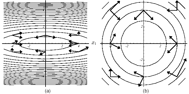
Figure 3.1-1. Example of vector pairs \(K\) -orthogonal in 2D: conditioning of \(K\) any (a), perfect conditioning (i.e. equal to unity) = usual orthogonality (b) .

We can therefore be satisfied with a linear combination of the type

\({d}^{i}:={r}^{i}+{\beta }^{i}{d}^{i-1}\) (3.1-3)

This is all the more so since it verifies the sufficient condition (2.3-4) and because of the orthogonality (2.3-3b), the following one-dimensional search (2.3-2) takes place in an optimal space: the plane formed by the two orthogonal directions \(({r}^{i},{d}^{i-1})\).

It therefore remains to determine the optimal value of the proportionality coefficient \({\beta }^{i}\). In the GC this choice is made in such a way as to maximize the attenuation factor of (2.3-4), that is to say the term

\(\frac{{\mathrm{\langle }{\mathrm{r}}^{\mathrm{i}},{\mathrm{d}}^{\mathrm{i}}\mathrm{\rangle }}^{2}}{\mathrm{\langle }{\mathrm{K}}^{\mathrm{-}1}{\mathrm{r}}^{\mathrm{i}},{\mathrm{r}}^{\mathrm{i}}\mathrm{\rangle }\mathrm{\langle }{\text{Kd}}^{i},{\mathrm{d}}^{\mathrm{i}}\mathrm{\rangle }}\) (3.1-4)

It leads to the expression

\({\beta }^{i}:=\frac{{\parallel {r}^{i}\parallel }^{2}}{{\parallel {r}^{i-1}\parallel }^{2}}\) (3.1-5)

and induces the same property of orthogonality of the successive residues as for the Steepest Descent (but without the zigzags!)

\(\langle {r}^{i},{r}^{i-1}\rangle =0\) (3.1-6)

A « residue-dd » condition is added

\(\langle {r}^{i},{d}^{i}\rangle ={\parallel {r}^{i}\parallel }^{2}\) (3.1-7)

which requires initializing the process*via* \({d}^{0}={r}^{0}\).

3.1.2. Algorithm

In short, by summarizing the relationships (2.2-5), (2.3-1), (2.3-1), (2.3-1), (2.3-3) and (3.1-3), (3.1-5), (3.1-7) the classical algorithm is obtained

\(\begin{array}{}\text{Initialisation}{u}^{0}\text{donné,}{r}^{0}={\text{f-Ku}}^{0},{d}^{0}={r}^{0}\\ \text{Boucle en}i\\ (1){z}^{i}={\text{Kd}}^{i}\\ (2){\alpha }^{i}=\frac{{\parallel {r}^{i}\parallel }^{2}}{\langle {d}^{i},{z}^{i}\rangle }(\text{paramètre optimal de descente})\\ (3){u}^{i+1}={u}^{i}+{\alpha }^{i}{d}^{i}(\text{nouvel itéré})\\ (4){r}^{i+1}={r}^{i}-{\alpha }^{i}{z}^{i}(\text{nouveau résidu})\\ (5)\text{Test d'arrêt via}\langle {r}^{i+1},{r}^{i+1}\rangle (\text{par exemple})\\ (6){\beta }^{i+1}=\frac{{\parallel {r}^{i+1}\parallel }^{2}}{{\parallel {r}^{i}\parallel }^{2}}(\text{paramètre de conjugaison optimal})\\ (7){d}^{i+1}={r}^{i+1}+{\beta }^{i+1}{d}^{i}(\text{nouvelle dd})\end{array}\)

Algorithm 4: Standard Conjugate Gradient (GC) .

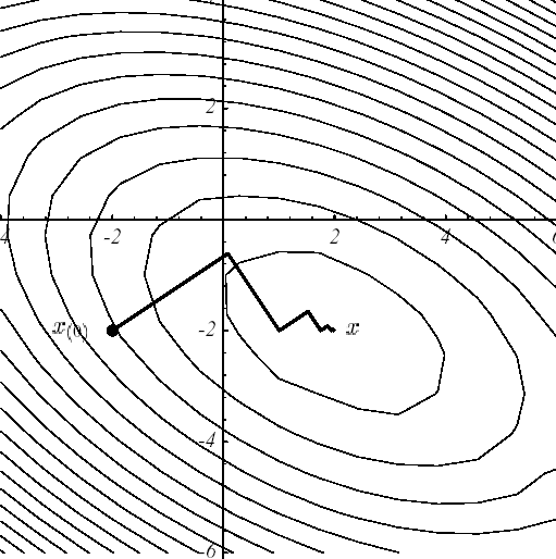
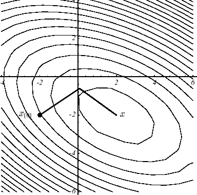
In example 1, the « supremacy » of the GC over the Steepest Descent is obvious (cf. figure 3.1-2) and is explained by the difference between the convergence result (2.2-9) and that of (3.2-9). In both cases, the same starting points and the same stopping criteria were chosen: \({u}^{0}={[-\mathrm{2,}-2]}^{T}\) and \({\parallel {r}^{i}\parallel }^{2}<\varepsilon ={\text{10}}^{-6}\).

hath

B

Figure 3.1-2. Comparative convergences, on example 1,

from Steepest Descent (a) and GC (b) .

Notes:

• This GC method was developed independently by M.R.Hestenes (1951) and E.Stiefel (1952) of the “National Bureau of Standard” in Washington D.C. (nursery of numericians with also C.Lanczos). The first theoretical results of convergence are due to the work of S.Kaniel (1966) and H.A.Van der Vorst (1986) and it was really popularized for solving large sparse systems by J.K.Reid (1971). The interested reader will find a commented history and an extensive bibliography on the subject in the papers by G.H.Golub, H.A Van der Vorst, and Y.Saad [Go89] [GV97] [] [SV00].

• For the record, thanks to its very wide distribution in the industrial and academic world, and, of its many variants, the GC was ranked third in the « Top10 » of the best algorithms of the XXe century [Ci00]. Just behind the Monte Carlo and simplex methods but in front of the **QR algorithm, Fourier transforms and multipole solvers!*

• Traces can be found in the GC’s EDF R&D codes from the beginning of the 1980s with the first work on the subject by J.P.Grégoire. Since then it has spread, with unequal happiness, in of many fields, _ N3S, Code_Saturn, COCCINELLE, Code_Aster, TRIFOU, ESTET, TELEMAC _, and it has been greatly optimized, vectorized, parallelized [Greg]…

• To the stop test on the residue norm, theoretically legitimate but in practice sometimes difficult to calibrate, we often prefer a dimensionless stopping criterion, such as the residue relating to the th iteration: \({\delta }^{i}:=\frac{\parallel {r}^{i}\parallel }{\parallel f\parallel }\) (see §5) .

3.2. Elements of theory

3.2.1. Krylov Space

By using the Petrov-Galerkin analysis already mentioned for Steepest Descent, we can summarize the action of the GC in one sentence. It carries out successive orthogonal projections on Krylov space \({\kappa }_{i}(K,{r}^{0}):=\text{vect}({r}^{0},{\mathrm{Kr}}^{0}\dots {K}^{i-1}{r}^{0})\) where \({r}^{0}\) is the initial residue: at the i th iteration \({K}_{i}={L}_{i}={\kappa }_{i}(K,{r}^{0})\). We solve the linear system (\({P}_{1}\)) by looking for an approximate solution \({u}^{i}\) in the affine subspace (search space with dimension \(N\))

\(A={r}^{0}+{\kappa }_{i}(K,{r}^{0})\) (3.2-1)

while imposing the orthogonality constraint (dimensional constraint space \(N\))

\({r}^{i}:=f-{\text{Ku}}^{i}\perp {\kappa }_{i}(K,{r}^{0})\) (3.2-2)

This Krylov space has the good property of facilitating the approximation of the solution, after \(m\) iterations, in the form

\({K}^{-1}f\approx {u}^{m}={r}^{0}+{P}_{m-1}(K)f\) (3.2-3)

where \({P}_{m-1}\) is a certain matrix polynomial of order \(m-1\). Indeed, it is shown that the residues and the directions of descent generate this space

\(\begin{array}{}\text{vect}({r}^{0},{r}^{1}\dots {r}^{m-1})={\kappa }_{m}(K,{r}^{0})\\ \text{vect}({d}^{0},{d}^{1}\dots {d}^{m-1})={\kappa }_{m}(K,{r}^{0})\end{array}\) (3.2-4)

while allowing the approximate solution, \({u}^{m}\), to minimize the energy standard over the entire affine space*A*

\({\parallel {u}^{m}\parallel }_{K}\le {\parallel u\parallel }_{K}\forall u\in A\) (3.2-5)

This result combined with the property (3.2-4b) illustrates all the optimality of the GC: unlike descent methods, the minimum amount of energy is not achieved successively for each direction of descent, but jointly for all the directions of descent already obtained.

Note:

• There is a wide variety of projection methods on Krylov-type spaces, more prosaically called « Krylov methods ». To solve linear systems [Saa03] (GC, GMRES,,, FOM,//IOM/DOM, GCR, ORTHODIR/MIN…) and/or modal problems [Boi01] (Lanczos, Arnoldi…). They differ in the choice of their constraint space and in that of the preconditioning applied to the initial operator to constitute the working operator, knowing that different implementations lead to radically different algorithms (vector or block version, orthonormalization tools, etc.).

3.2.2. Orthogonality

As already mentioned, the descent directions are \(K\) -orthogonal to each other. Moreover, the choice of the optimal descent parameter (cf. (2.2-4), (2.2-4), (2.2-4), (2.3-3a) or step (2)) imposes, step by step, the orthogonalities

\(\begin{array}{}\langle {d}^{i},{r}^{m}\rangle =0\forall i<m\\ \langle {r}^{i},{r}^{m}\rangle =0\end{array}\) (3.2-6)

We therefore note a small approximation in the name of the GC, because the gradients are not conjugate (cf. (3.2-6b)) and the conjugated directions do not only include gradients (cf. (3.1-3)). But let’s not « quibble », the designated ingredients are still there!

At the end of \(N\) iterations, two scenarios arise:

• Let the residue be zero \({r}^{N}=0\) so convergence.

• Or it is orthogonal to the previous \(N\) directions of descent which constitute a base of the finite space of approximation \({\Re }^{N}\) (as they are linearly independent). Hence, necessarily, \({r}^{N}=0\), so convergence.

So it seems that GC is a direct method that converges in at most \(N\) iterations, at least that’s what we believed before testing it on practical cases! Because what remains true in theory, in exact arithmetic, is undermined by the finite arithmetic of calculators. Progressively, especially because of rounding errors, the directions of descent lose their beautiful conjugation properties and the minimization goes out of the required space.

In other words, we solve an approximate problem that is no longer quite the desired projection of the initial problem. The (theoretically) direct method has revealed its true nature! It is iterative and therefore subject, in practice, to numerous hazards (conditioning, starting point, stopping tests, precision of orthogonality, etc.).

To remedy this, a reorthogonalization phase can be imposed during the construction of the new descent direction (cf. algorithm 4, step (7)). This very widespread practice in modal analysis [Boi01] and annex 2) and in domain decomposition [Boi08] can be used in different variants: total, partial, selective reorthogonalization… via a whole range of orthogonalization procedures (GS, GSM, IGSM, Househölder, Givens).

These reorthogonalizations require, for example, the storage of the first \({N}_{\mathrm{orth}}\) vectors \({d}^{k}(k=1\dots {N}_{\text{orth}})\) and their product by the work operator \({z}^{k}={\mathrm{Kd}}^{k}(k=1\dots {N}_{\text{orth}})\). Formally, it is therefore a question of substituting the following calculation for the last two steps of the algorithm

\({d}^{i+1}={r}^{i+1}-\sum _{k=0}^{\text{max}(i,{N}_{\text{orth}})}\frac{\langle {r}^{i+1},{\text{Kd}}^{k}\rangle }{\langle {d}^{k},{\text{Kd}}^{k}\rangle }{d}^{k}(\text{nouvelle dd}K-\text{orthogonalisée})\) (3.2-7)

Through the various digital experiments that have been carried out (cf. in particular the work of J.P.Grégoire and [Boi03]), it seems that this reorthogonalization is not always effective. Its additional cost due mainly to the new matrix-vector \(K{d}^{k}\) products (and their storage) is not always offset by the gain in the number of global iterations.

3.2.3. Convergence

Because of the particular structure of the approximation space (3.2-3) and the property of minimization on this space of the approximate solution \({u}^{m}\) (cf. (3.2-5)), we obtain an estimate of the convergence speed of the GC

\(\begin{array}{}{\parallel e({u}^{i})\parallel }_{K}^{2}={({\omega }^{i})}^{2}{\parallel e({u}^{0})\parallel }_{K}^{2}\\ \text{avec}{\omega }^{i}:=\underset{1\le i\le N}{\text{max}}(1-{\lambda }_{i}{P}_{m-1}({\lambda }_{i}))\end{array}\) (3.2-8)

where we denote \(({\lambda }_{i};{v}_{i})\) the eigenmodes of the \(K\) matrix and \({P}_{m-1}\) any polynomial of degree at most \(m-1\). The famous Tchebycheff polynomials, via their good increase properties in the polynomial space, make it possible to improve the readability of this attenuation factor \({\omega }^{i}\) . At the end of \(i\) iterations, at worst, the decrease is then expressed in the form

\({\parallel e({u}^{i})\parallel }_{K}\le 2{(\frac{\sqrt{\eta (K)}-1}{\sqrt{\eta (K)}+1})}^{i}{\parallel e({u}^{0})\parallel }_{K}\) (3.2-9)

It ensures the superlinear convergence (i.e. \(\underset{i\to \infty }{\text{lim}}\frac{J({u}^{i+1})-J(u)}{J({u}^{i})-J(u)}=0\)) of the process in a number of iterations that is proportional to the square root of the operator’s conditioning. So, in order to get

\(\frac{{\parallel e({u}^{i})\parallel }_{K}}{{\parallel e({u}^{0})\parallel }_{K}}\le \varepsilon (\text{petit})\) (3.2-10)

You need a number of iterations in the order of

\(i\approx \frac{\sqrt{\eta (K)}}{2}\text{ln}\frac{2}{\varepsilon }\) (3.2-11)

Obviously, as we have noted many times, a poorly conditioned problem will slow down the convergence of the process. But this slowdown will be less noticeable for the GC than for the Steepest Descent (cf. figures 3.2-1). And anyway, the overall convergence of the former will be better.

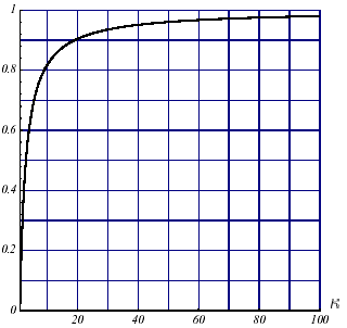
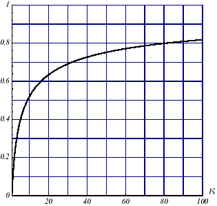
Figure 3.2-1. Comparative convergences of the Steepest Descent

(a) and GC (b) (to the nearest factor of ½) depending on conditioning \(\kappa\) .

Notes:

• In practice, taking advantage of particular circumstances, _ better starting point and/or advantageous spectral distribution _, the convergence of the GC may be much better than expected (3.2-9). Since Krylov’s methods tend to identify extreme eigenvalues primarily, the « effective conditioning » of the work operator is improved.

• On the other hand, some iterations of the Steepest Descent may provide a better decrease in the residue than the same iterations of the GC. Thus, the first iteration of the GC is identical to that of the Steepest-Descent and therefore with an equal convergence rate.

3.2.4. Complexity and memory occupancy

As with the Steepest Descent, most of the computational cost of this algorithm lies in step (1), the matrix-vector product. Its complexity is of the order of \(\Theta (\text{kcN})\) where \(c\) is the average number of non-zero terms per line of \(K\) and \(k\) is the number of iterations required at convergence. To be much more effective than a simple Cholesky (of complexity \(\Theta (\frac{{N}^{3}}{3})\)) you must therefore:

Take into account the hollow nature of matrices resulting from finite element discretizations (storage MORSE, optimized matrix-vector product*ad hoc): \(c\text{<<}N\).

• Precondition the work operator: \(k\text{<<}N\).

It has already been pointed out that for an operator SPD its theoretical convergence occurs in, at most, \(N\) iterations and in proportion to the root of the conditioning (cf. (3.2-11)). In practice, for large systems that are poorly conditioned (as is often the case in structural mechanics), it can be very slow to occur (cf. Lanczos phenomenon in the following paragraph).

Taking into account the conditions of operators generally observed in structural mechanics and recalled for the study of the complexity of the Steepest Descent, whose notations are taken from, the computational complexity of the GC is written \(\Theta ({\text{cN}}^{\frac{1}{d}+1})\) (resp. \(\Theta ({\text{cN}}^{\frac{2}{d}+1})\)).

As for memory occupancy, as for the Steepest Descent, only the storage of the working matrix is possibly required: \(\vartheta (\text{cN})\). In practice, the computer implementation of sparse storage requires the management of additional integer vectors: for example for the MORSE storage used in Code_Aster, vectors of the end of line indices and column indices of the elements of the profile. Hence an effective memory complexity of \(\Theta (\text{cN})\) real and \(\vartheta (\text{cN}+N)\) integers.

Note:

• These memory congestion considerations do not take into account the storage problems of a possible preconditioner and the workspace that its construction may temporarily require.

3.3. Complements

3.3.1. Equivalence with the Lanczos method

By « triturating » the orthogonality property of the residue with any vector of Krylov space (cf. (3.2-2)), we show that the \(m\) iterations of the GC lead to the construction of a Lanczos factorized of the same order (cf. [Boi01] §5.2)

\({\text{KQ}}^{m}\mathrm{=}{\mathrm{Q}}^{\mathrm{m}}{\mathrm{T}}^{\mathrm{m}}\mathrm{-}\underset{{\mathrm{R}}^{\mathrm{m}}}{\underset{\underbrace{}}{\frac{\sqrt{{\beta }^{m}}}{{\alpha }^{m\mathrm{-}1}}{\mathrm{q}}^{\mathrm{m}}{\mathrm{e}}_{\mathrm{m}}^{\mathrm{T}}}}\) (3.3-1)

by noting:

• \({R}^{m}\) the specific « residue » of this factorization,

:math:`{e}_{m}` the*m th vector of the canonical base,

• \({q}^{i}:=\frac{{r}^{i}}{\parallel {r}^{i}\parallel }\) the residue vectors standardized to the unit, called for the occasion Lanczos vectors,

• \({Q}^{m}:=\left[\begin{array}{ccc}\frac{{r}^{0}}{\parallel {r}^{0}\parallel }& \dots & \frac{{r}^{m-1}}{\parallel {r}^{m-1}\parallel }\end{array}\right]\) the orthogonal matrix they constitute.

m

m

Figure 3.3-1. Lanczos factorization induced by the GC.

The Rayleigh matrix, which expresses the orthogonal projection of \(K\) onto Krylov \({\kappa }_{m}(K,{r}^{0})\) space, then takes the canonical form.

\({T}^{m}=\left[\begin{array}{cccc}\frac{1}{{\alpha }^{0}}& -\frac{\sqrt{{\beta }^{1}}}{{\alpha }^{0}}& 0& 0\\ -\frac{\sqrt{{\beta }^{1}}}{{\alpha }^{0}}& \frac{1}{{\alpha }^{1}}+\frac{{\beta }^{1}}{{\alpha }^{0}}& \text{.}\text{.}\text{.}& 0\\ 0& \text{.}\text{.}\text{.}& \text{.}\text{.}\text{.}& -\frac{\sqrt{{\beta }^{m-1}}}{{\alpha }^{m-2}}\\ 0& 0& -\frac{\sqrt{{\beta }^{m-1}}}{{\alpha }^{m-2}}& \frac{1}{{\alpha }^{m-1}}+\frac{{\beta }^{m-1}}{{\alpha }^{m-2}}\end{array}\right]\) (3.3-2)

Almost without additional calculation, the GC thus provides the Rayleigh approximation of the work operator in a sympathetic form, _ tridiagonal symmetric square matrix of adjustable size _, from which it will be easy to deduce the spectrum (via, for example, a robust QR, for example, a robust QR, cf. [Boi01] appendix 2)).

At the end of a linear system inversion conducted by a simple GC, it is therefore possible, at a lower cost, to know, in addition to the solution sought, an approximation of the spectrum of the matrix and therefore of its conditioning [Greg]. This feature could be inserted in*Code_Aster* in order to better control the preconditioning level.

Notes:

• Since the work operator is SPD, its Rayleigh matrix inherits this property and its decomposition is directly obtained \({T}^{m}={L}^{m}{D}^{m}{({L}^{m})}^{T}\) with

\({L}^{m}:=\left[\begin{array}{cccc}1& 0& 0& 0\\ -\sqrt{{\beta }^{1}}& 1& \text{.}\text{.}\text{.}& 0\\ 0& \text{.}\text{.}\text{.}& \text{.}\text{.}\text{.}& 0\\ 0& 0& -\sqrt{{\beta }^{m-1}}& 1\end{array}\right]\text{et}{D}^{m}:=\left[\begin{array}{cccc}\frac{1}{{\alpha }^{0}}& 0& 0& 0\\ 0& \frac{1}{{\alpha }^{1}}& \text{.}\text{.}\text{.}& 0\\ 0& \text{.}\text{.}\text{.}& \text{.}\text{.}\text{.}& 0\\ 0& 0& 0& \frac{1}{{\alpha }^{m-1}}\end{array}\right]\) (3.3-3)

Since the Lanczos method does not calculate these intermediate terms \({\alpha }^{i}\) and \({\beta }^{i}\) , but directly *the tridiagonal terms, it does not have access to this information. On the other hand, it can take into account**symmetric matrices that are not necessarily positive definite. *

• So, whether it is a question of inverting a linear system or determining a part of its spectrum, these Krylov methods work on the same principle: progressively determine the base vectors generating the projection space at the same time as the result of this projection. In the GC as in Lanczos, we strive to make this projection the most robust (orthogonality of the base vectors), the smallest (projection size = number of iterations) and the simplest possible (orthogonal projection). For the modal solver, another constraint is juxtaposed: to approximate the spectrum of the work operator as best as possible by that of the Rayleigh matrix. In non-symmetric, we speak of a projection that is no longer orthogonal but oblique and the approximations then take place between GMRES and Arnoldi.

• In exact arithmetic, after of \(N\) iterations, we have completely determined the entire spectrum of the operator. In practice, rounding and orthogonalization problems prevent us from doing so. But, if you are patient enough ( \(m\gg N\)), you are still able to detect the whole spectrum: this is what we call the Lanczos phenomenon (cf. [Boi01] §5.3.1/5.3.3).

• *Paradoxically, the loss of orthogonality is mainly due to the convergence of an eigenmode rather than to rounding errors! This analysis due to CC.Paige (1980) attests that as soon as an eigenmode is captured it disrupts the orthogonal arrangement of the Lanczos vectors (in the case we are concerned with, the residuals and the directions of descent). In modal terms, the digital treatment of this parasitic phenomenon has**the subject of numerous palliative developments. As for the GC, it must limit the effectiveness of the methods of reorthogonalization of the directions of descent mentioned above. *

3.3.2. Nested solvers

As already noted, linear solvers are often buried deep within other algorithms, and in particular, Newtons-type nonlinear solvers. For the*Code_Aster*, these are the most frequently used application cases: operators STAT_NON_LINE, DYNA_NON_LINE and THER_NON_LINE.

In such a configuration, a linear solver such as the GC can do well (compared to a direct solver). Its iterative nature is useful for making the algorithm stop test evolve (cf. step (5) algorithm 4) according to the relative error of the nonlinear solver that encapsulates it: this is the problem nested solvers (we also talk about relaxation) [CM01] [GY97] [BFG] [] [] [] whose CERFACS is the « spearhead » in France.

By relaxing the required precision on the cancellation of the residue at the appropriate time (for example strategy in the case Krylov + GC modal method) or, on the contrary, by hardening it (resp. power modal method + Gauss-Seidel + GC), we can thus gain in complexity calculation on the GC without modifying the convergence of the global process. Of course, simple and inexpensive criteria must be developed for the gain to be substantial. This feature could be inserted in*Code_Aster* (internal and automatic control of the RESI_RELA value).

Note:

• Some authors have also asked themselves the question of the order in which these algorithms are linked: « Newton—GC » or « GC-Newton »? Although from a computer and conceptual point of view, the question is quickly resolved: we prefer the first solution, which is more readable, more flexible and which does not disturb the existing one, from a numerical and algorithmic point of view, sharing is more nuanced. This may depend on the « technical triplows » deployed by the non-linear solver (tangent matrix, one-dimensional minimization…) and on the GC deployed (preconditioner). Nevertheless, it seems that the natural order, « Newton—GC », is the most efficient and the most scalable.

3.3.3. Parallelism

Like many iterative solvers, GC lends itself well to parallelism. It’s quite scalable [23] _ . The main elementary operations that constitute it (matrix-vector product, typical operation [24] _ « daxpy and dot product) break down efficiently between different processors, only parallelizing the preconditioner (often based on a direct solver) can be difficult (problems often referred to as: “parallel preconditioning”). Moreover, linear algebra libraries (PETSc, HYPRE, TRILINOS…) do not always offer a parallel version of their preconditioners. Concerning preconditioners, we therefore have two criteria that tend to contradict each other: parallel efficiency and algorithmic efficiency.

Codes therefore tend to favor preconditioners that are not very effective from an algorithmic point of view [25] _ (Jacobi type) but not very memory-intensive and very parallelizable. The parallel gain (called speed-up) is very interesting right away, but the sequential point of comparison may not be very glorious [26] _ !

Another difficulty with parallelism also comes from the distribution of data. Care must be taken to ensure that the various rules that govern the calculation data (allocation of boundary condition zones, allocation of materials, choice of finite elements, etc.) are not affected by the fact that each processor only partially knows them. This is called the « consistency » of distributed data [BOI08b].

Likewise, ad hoc communications must be provided in the code during each global manipulation of data (stopping criteria, post-processing, etc.).

Notes:

• Thus on machine CRAY, J.P.Grégoire [Greg] adapted and parallelized, in shared memory and in distributed memory, a preconditioned conjugate gradient algorithm. Four types of operations are carried out concurrently: elementary vector operations, dot products, matrix-vector products and the construction of the preconditioner (diagonal). Parallel preconditioning problems, which were only resolved for the diagonal preconditioner, unfortunately did not allow these models to be ported to the official version of Code_Aster.

• Direct solvers and other iterative solvers (Gauss-Seidel stationary methods, SSOR..) are considered to be less scalable than Krylov methods (GC, GMRES…) .

In fact, we are now going to address the thorny issue of preconditioning for GC. It will then become the Preconditioned Conjugate Gradient: GCPC.

[1]

The Fletcher-Reeves and Polak-Ribière methods (cf. §2.3) are also part of this family of methods.

[2]

Or extensibility in French. A method is said to be scalable from a strong point of view (this is the criterion by default, “strong scalability”), if it makes it possible to solve a problem all the more quickly as processors are added proportionally. Less commonly, we speak of “weak scalability”, when it comes to solving, in a comparable amount of time, a bigger problem by increasing the number of processors by the same amount of time (cf. [Boi08] §2.4).

[3]

To use terminology specific to the BLAS library. An operation like DAXPY makes linear combinations of vectors.

[4]

Going so far as to tolerate convergence in thousands of iterations.

[5]

Strictly speaking, to express a parallel gain, one should take the best sequential calculation as a reference. The latter using a more effective and possibly sequential preconditioner. However, the exercise raises a difficulty: this operating point is often difficult to demonstrate. The size of the studies, taking into account the hardware characteristics of the machines, immediately require a calculation distributed over dozens of processors!