5. Algorithmic resolution — Frictionless contact#
5.1. Contact links#
Each slave node potentially in contact has a status whose nature the algorithms will have to determine. A slave node is called a « potential contact link » or more simply « link ». The term connection alludes to the fact that the contact condition is the result of the imposition of a kinematic relationship on the degrees of liberty of movement of the slave node. These connections are combined in different sets:
:math:`` is the set of possible links (active and non-active);
\({\Xi }^{\text{nc}}\) is the set of slave nodes that are not in contact (links not active);
\({\Xi }^{\text{c}}\) is the set of nodes actually in contact (active links).
We therefore have the following relationships between the sets:
\({\Xi }^{\text{c}}\mathrm{\cap }{\Xi }^{\text{nc}}\mathrm{=}\mathrm{\varnothing }\) because the nodes are in contact or not;
\({\Xi }^{\text{l}}\mathrm{=}{\Xi }^{\text{c}}\mathrm{\oplus }{\Xi }^{\text{nc}}\) because the nodes that are potentially in contact are or are not in contact;
5.2. Dualized methods in contact#
5.2.1. Balance of the structure in the presence of contact#
Recall that the equilibrium equation in the presence of contact is written as:
: label: eq-102
left{{L} _ {i} ^ {text {int}}} ({u} _ {int}}} ({u} _ {i})rightmathrm {=}left{{L} _ {i} _ {i} ^ {i} ^ {i} ^ {text {ext}}} ^ {text {ext}}}} ({u} _ {ext}}} ^ {u} _ {ext}}} ({u} _ {i}}} ({u} _ {i}}) ({u} _ {i}}) ({u} _ {i}}) ({u} _ {i}}) ({u} _ {i}}) ({u} _ {i}})right}mathrm {-}}}right}
In the case of dual contact, the contact force is written according to the contact Lagrange multiplier:
: label: eq-103
left{{L} _ {i} ^ {text {c}}right}right}right}mathrm {=} {left{{L} _ {i} ^ {text {c}}right}}rightright}}} {text {c}}}} {text {c}}}} _ {text {c}}}} _ {text {c}}}} _ {text {dual}}} _ {text {dual}}} _ {text {dual}}} _ {text {dual}}} _ {text {dual}}}mathrm {=}}mathrm {=} {mathrm {A} ^ {text {c}}}rightright}} ^ {T}mathrm {.} left{{mu} _ {i} ^ {text {c}}right}
After linearization of the equilibrium equation (), we introduce the tangent matrix \(\left[{K}^{\text{m},n\mathrm{-}1}\right]\) which will contain the contributions resulting from the linearization of internal and external forces and the matrix \(\left[{K}^{\text{c},n\mathrm{-}1}\right]\) for contact forces, we find \(\left\{\delta {\tilde{u}}^{n}\right\}\), increment of solution of the balance problem at iteration \(n\) but without application of the law of contact:
: label: eq-104
(left [{K} ^ {text {m}, nmathrm {-} 1}right] +left [{K} ^ {text {c}, nmathrm {-} 1} 1}right])mathrm {.} left{delta {tilde {u}}} ^ {n}right} ^ {n}right}mathrm {=}left{{L} _ {i} ^ {text {int}, nmathrm {-}}mathrm {-}}left{{L} _ {i} ^ {text {int}, nmathrm {-}, nmathrm {-} 1}}rightright}}rightright}}mathrm {-}left{{L} _ {i} ^ {text {int}, nmathrm {-} 1} 1}rightright}right}}rightright}}mathrm {-}} 1}right} +left{{L} _ {i} ^ {text {c}, nmathrm {-} 1}right}
We have seen that the contact forces in the dual case do not depend on displacement (see § 4.3.5). So we have \(\left[{K}^{\text{c},n\mathrm{-}1}\right]\mathrm{=}0\). This allows us to express the balance of the structure taking into account contact forces (noting \(\left[K\right]\mathrm{=}\left[{K}^{\text{m},n\mathrm{-}1}\right]\) and \(\left\{F\right\}\mathrm{=}\left\{{L}_{i}^{\text{ext},n\mathrm{-}1}\right\}\mathrm{-}\left\{{L}_{i}^{\text{int},n\mathrm{-}1}\right\}\mathrm{-}\left\{{L}_{i}^{\text{c},n\mathrm{-}1}\right\}\) to lighten):
: label: eq-105
left [Kright]mathrm {.} left{delta {tilde {u}}} ^ {n}right}mathrm {=}left{Fright}
Solution \(\left\{{\tilde{u}}_{i}^{n}\right\}\) is obtained after equilibrium and before applying contact conditions. It is written:
: label: eq-106
left{{tilde {u}} _ {i}} _ {i} ^ {n}right}mathrm {=}left{{u} _ {imathrm {-} 1}right}right}}}right}right}right}right}}right}right}right}right}}right}right}}right}}right}right}}right}right}}right}}right}right}}right}}right}right}}right}}right}right}}right}}right}right}}right} {u}} ^ {n}right}
To get solution \(\left\{{\tilde{u}}_{i}^{n}\right\}\), we did not apply the contact conditions (Signorin’s law) for the current Newton iteration \(n\). On the other hand, the contact reactions calculated at the previous Newton iteration \(n\mathrm{-}1\) are well taken into account in \(\left\{F\right\}\). To completely solve the balance problem with touch/friction, in iteration \(n\), we must apply the law of Signorin, which is expressed by the following system:
: label: eq-107
mathrm {{}begin {array} {cc} {cc}left [{A} ^ {text {c}}right]text {.} left{{u} _ {i} ^ {n}right}right}mathrm {le}left{{d} _ {text {ini}} ^ {text {c}}right}right}right}right}rightright}rightright}rightright}rightright}rightright}right\ right}right}right\ right}right}right\ right}right}right\ right}right}right}right\ right}right}right\ right}right}right\ right}right}right\ right}rightb)\ langle {mu} _ {i} ^ {text {c}}ranglemathrm {.} (left [{A} ^ {text {c}}}right]mathrm {.} left{{u} _ {i} ^ {n}right})mathrm {=} 0& (c)end {array}
We recall the interpretation of the Signorin conditions:
Equation (a) represents the geometric conditions of non-interpenetration, the inequality being understood component by component (each line relates to a potential contact couple).
Equation (b) expresses the absence of opposition to detachment (contact surfaces can only experience compressions), this is the so-called intensity condition.
Equation (c) is the compatibility condition. When for a given link the Lagrange multiplier is non-zero, there is contact and therefore the game is zero. When the game is non-zero (the two surfaces are not in contact), the associated multiplier must be zero (no compression).
The application of Signorin’s law will modify the displacement increment \(\left\{\delta {\tilde{u}}^{n}\right\}\) (which becomes \(\left\{\delta {u}^{n}\right\}\)), hence the solution obtained after balance and after application of the contact law which is written:
: label: eq-108
left{{u} _ {i} ^ {n}right}right}right}mathrm {=}left{{u} _ {imathrm {-} 1}right}} +left} +left{delta {u}} +left{delta {u}} +left{delta {u} {u}left{delta {u} {u} +left{delta {u} {u}left{delta {u} {u}left{delta {u} {u}right}
5.2.2. System reduced to active links#
We are going to write the system to completely solve the balance problem taking into account the law of Signorin. The idea is to transform the inequalities of the system () into equalities. We start by evaluating the game given by the displacement calculated before the correction of contact \(\left\{{\tilde{d}}^{\text{c},n}\right\}\), for all the connections [bib7] _ 5.1 :
: label: eq-109
{left{{tilde {d}}} ^ {text {c}}} ^ {text {c}}} ^ {text {l}}}mathrm {=} {\ left{{d}} _ {text {d}} _ {text {d}} _ {text {ini}}}} ^ {text {c}}right}mathrm {-} {-}left [{A} ^ {text {c}}right]mathrm {.} (left{{u} _ {imathrm {-} 1}right} 1}right} +left{Delta {u} _ {i} ^ {nmathrm {-} 1}right} 1}right}} +leftmathrm {-} - {-} 1}right}} +leftmathrm {-} 1}right}} +left{delta {-} -} 1}right}} +left{delta {-} -} 1}right}} +left{delta {-} -} 1}right}} +left{delta {-} -} 1}right}} +left{delta {-}
We say that a link \(J\) is active if its game \({⌊\left\{{\tilde{d}}^{\text{c},n}\right\}⌋}_{\text{J}\mathrm{\in }{\Xi }^{\text{l}}}\) is negative, which indicates an interpenetration (the contact condition is not respected), this link therefore becomes a contact link and therefore makes it possible to define the initially postulated set of contact links \({\Xi }^{\text{c}}\):
: label: eq-110
{Xi} ^ {text {c}}mathrm {=}left{=}left{Jmathrm {in} {xi} ^ {text {l}}mathrm {mid} {mid} {{}} {mid} {} {} {} {} {left} {} {leftleft}left{d}} ^ {{tilde {d}}} ^ {text {c}} ^ {right}
It is postulated that, for these active links, the effective game will be zero, and that therefore inequality \({⌊\left[{A}^{\text{c}}\right]\mathrm{.}\left\{{u}_{i}^{n}\right\}⌋}_{{\Xi }^{\text{l}}}\mathrm{\le }{⌊\left\{{d}_{\text{ini}}^{\text{c}}\right\}⌋}_{{\Xi }^{\text{l}}}\) becomes an equality for all active links:
: label: eq-111
{left [{A} ^ {text {c}}}right]mathrm {.} left{{u} _ {i} ^ {n}right}right}mathrm {=}left{{d} _ {text {ini}} ^ {text {c}}right}}right}}right}}right}}
If we use \(\left\{{d}^{\text{c},n\mathrm{-}1}\right\}\), the game evaluated before the current Newton iteration:
: label: eq-112
left{{d} ^ {text {c}}, nmathrm {-} 1}right}rightmathrm {=}left{{d} _ {text {ini}}}} ^ {text {ini}}}} ^ {text {ini}}}} ^ {text {ini}}}} ^ {text {ini}}}} ^ {text {ini}}}} ^ {text {ini}}} ^ {text {ini}}} ^ {text {ini}}} ^ {text {ini}}} ^ {text {ini}}} ^ {text {ini}}} ^ {text {ini}}} ^ {text {ini}}} ^ {text {ini}}} ^ { (left{{u} _ {imathrm {-} 1}right} +left{Delta {u} _ {i} ^ {nmathrm {-} 1}right})
With:
Equality () is finally written:
: label: eq-114
{left [{A} ^ {text {c}}}right]mathrm {.} left{delta {u} ^ {n}right}right}mathrm {=}left{{d} ^ {text {c}, nmathrm {-} 1}right} 1}right}}right}
The « mixed » inequality/equality system (containing the equilibrium equation and the Signorin conditions) is finally transformed into a simple system that only treats equality, based on the contact links postulated \({\Xi }^{\text{c}}\):
: label: eq-115
mathrm {{}begin {array} {c} {c}left [Kright]mathrm {.} left{delta {u} ^ {n}right}right} +mathrm {[} {A} ^ {text {c}} {mathrm {]}}}} ^ {n}rightrightright} +mathrm {.} left{{mu} _ {i} ^ {text {c}} {text {c}}right}mathrm {=}left{Fright}\ {left [{A}left [{A} ^ {A} ^ {text {c}}}right]mathrm {.} left{delta {u} ^ {n}right} {n}right}mathrm {=}left{{d} ^ {text {c}, nmathrm {-} 1}right} 1}right}}right}}right}
We are looking for the unknowns \(\left\{\delta {u}^{n}\right\}\) and \(\left\{{\mu }_{i}^{\text{c}}\right\}\) which are solutions to the following system:
: label: eq-116
left [begin {array} {cc}mathrm {[}}mathrm {[}} Kmathrm {]}} &mathrm {[} {c}} {mathrm {]}}}} ^ {T}}} ^ {T}}\ mathrm {[}}}} ^ {T}\ mathrm {[}}}} ^ {T}\ mathrm {[}}}} ^ {T}\ mathrm {[}} 0mathrm {]}end {array}right]mathrm {.} left{begin {array} {c}left{delta {u}left{c}}\ text {c}} ^ {c}}right}right}right}right}left}end {array}right}right}right}right}right}left{{d} ^ {text {c}, nmathrm {-} 1}right}end {array}right}mathrm {iff}left [{K}}left [{K}}left [{K}} ^ {text {c}}right]mathrm {.}left [{K}}left [{K}} ^ {text {c}}right]mathrm {.} left{begin {array} {c}left{delta {u}left{c}}\ text {c}} ^ {c}}right}right}right}right}left}end {array}right}right}right}right}right}left{{d} ^ {text {c}, nmathrm {-} 1}right}end {array}right}
It will be noted that the dualized formulation of the non-interpenetration condition reflects the stationarity of the Lagrangian \(L\) thus defined:
: label: eq-117
L (left{delta {u} ^ {n}right},left{{mu} _ {i} ^ {text {c}}right})mathrm {=}right})mathrm {=}}frac {1} {2}mathrm {.} langledelta {u} ^ {n}ranglemathrm {.} left [Kright]mathrm {.} left{delta {u} ^ {n}right}right}mathrm {-}langledelta {u} ^ {n}ranglemathrm {.} left{Fright} +langle {mu} _ {i} ^ {text {c}}ranglemathrm {.} (left [{A} ^ {text {c}}}right]mathrm {.} left{delta {u} ^ {n}right} {n}right}mathrm {-}left{{d} ^ {text {c}, nmathrm {-} 1}right})
This stationarity is expressed in the form of the saddle point problem:
5.2.3. The active constraints method — ALGO_CONT =” CONTRAINTE “#
The aim is to generalize the approach in the previous paragraph by adopting an iterative algorithm that works in three phases:
Make hypotheses about the state of relationships (transformations inequalities → equality);
Solving the new system thus created;
Check the initial hypotheses and complete (possibly) in 1.
A complete description of the method with the necessary theoretical justifications can be found in [bib2] _ and [bib2] _. The principle is as follows: we postulate a set of so-called active constraints, which correspond to a zero game (the inequality relationship becomes an equality); we solve the system of equations obtained in this subspace, and we see if the initial postulate was justified. If the selected set was too small (active links had been forgotten), the link that most violates the non-interpenetration condition is added to the set; if the selected set was too large (links that are supposed to be active are in fact not active), the most improbable link is removed from the set i.e. the one whose Lagrange multiplier violates the intensity condition the most. Removing or adding a single link at each iteration of the method guarantees convergence into a finite number of iterations less than or equal to twice the maximum number of links, provided that the \(\left[K\right]\) matrix is symmetric and positive definite [1] _, [bib15] _, [bib16] _, [bib16] _.
In elasticity, at the end of the active stress iterations, we have a converged result in the Newton sense. In plasticity or if we update the geometry, this is not the case because several Newton iterations are necessary to obtain balance. After each Newton iteration, the active constraints algorithm is launched to satisfy the contact conditions. Thus, in terms of elasticity, we will necessarily converge for each step in one iteration if REAC_GEOM =” SANS “.
5.2.3.1. Writing the iterative problem#
We start from the increment obtained without processing the contact \(\left\{\mathrm{\delta }{\stackrel{~}{u}}^{n}\right\}\) and we perform the iterations of active constraints \(k\) until the proper convergence of this algorithm is achieved. Convergence in the sense of active constraints is obtained when no link violates the kinematic condition (inequality (a)) and when the associated Lagrange multipliers are all positive (inequality (b)).
Note \(k\) active constraint iterations. The starting solution without contact correction is \(\left\{\delta {\tilde{u}}^{n}\right\}\) and the increment added by the new contact iteration is \(\left\{{\delta }_{k}\right\}\). We note:
We are on the contact iteration \(k\). We are trying to solve the system ():
Note that the Lagrange multiplier for contact \(\left\{{\mu }_{i}^{\text{c}}\right\}\) is not solved incrementally but in a total way (over the time step). By injecting () into this system, we obtain:
: label: eq-121
mathrm {{}begin {array} {c} {c}left [Kright]mathrm {.} left{delta {u} _ {kmathrm {-} 1} ^ {n}right} +left [Kright]mathrm {.} left{{delta} _ {k}right}} +mathrm {[} {A} _ {k} ^ {text {c}} {mathrm {]}} {mathrm {]}}}} ^ {T}mathrm {.} left{{mu} _ {i} ^ {text {c}} {text {c}}right}mathrm {=}left{Fright}\ {left [{A} _ {k} _ {k}} ^ {text {c}}right]mathrm {.} (left{delta {u} _ {kmathrm {-} 1}} ^ {n}right} +left{{delta} _ {k}right})mathrm {=}}left{{d}left{{d}} ^ {{d} ^ {text {d} ^ {text {c} ^ {text {c}} ^ {text {c}}, nmathrm {-} 1}right}}} _ {xi} _ {k} _ {k}} ^ {text {c}}}}end {array}
The first equation can be rewritten:
: label: eq-122
left{{delta} _ {k}right}right}mathrm {=} {left [Kright]} ^ {mathrm {-} 1}mathrm {-} 1}mathrm {.} left{Fright}mathrm {-}left{delta {u} _ {kmathrm {-} 1} ^ {n}right}mathrm {-}mathrm {-} {-} {left [Kright]} {left [Kright]}} ^ {mathrm {-} 1}mathrm {-} 1}mathrm {-} 1}mathrm {-} mathrm {[} {A} _ {k} ^ {text {c}} {mathrm {]}}} ^ {T}mathrm {.} left{{mu} _ {i} ^ {text {c}}right}
Taking into account that \(\left\{\delta {\tilde{u}}^{n}\right\}\mathrm{=}{\left[K\right]}^{\mathrm{-}1}\mathrm{.}\left\{F\right\}\), we simplify:
From the postulated state of active links:
And using the \(\left\{{d}^{\text{c},n\mathrm{-}1}\right\}\) expression given by ():
: label: eq-125
{left [{A} _ {k} ^ {text {c}}right]mathrm {.} left{delta {u} _ {kmathrm {-} 1} ^ {n}right} +left [{A} _ {k} ^ {text {c}} ^ {text {c}}right]mathrm {.} left{{delta} _ {k}right}right}}} _ {{xi} _ {C} ^ {k}}mathrm {=} {left{{d} _ {text {d} _ {text {ini}}}} ^ {text {ini}}}} ^ {text {ini}}}} ^ {text {ini}}} ^ {text {ini}}} ^ {text {ini}}} ^ {text {ini}}} ^ {text {ini}}} ^ {text {ini}}} ^ {text {ini}}} ^ {text {ini}}} ^ {text {ini}}} ^ {text {ini}}} ^ {text {ini}}} ^ right]text {.} (left{{u} _ {imathrm {-} 1}right} 1}right} +left{Delta {u} _ {i} ^ {nmathrm {-} 1}right})right}})}} _ {xi} _ {xi} _ {k} _ {k} _ {text {c}}}}
We use the \(\left\{{\delta }_{k}\right\}\) expression given by ():
In the end, the Lagrange multipliers \(\left\{{\mu }_{i}^{\text{c}}\right\}\) for contact links are solutions of the following system:
: label: eq-127
{mathrm {-}left [{A} _ {k} _ {k} ^ {text {c}}right]mathrm {.} {left [Kright]} ^ {mathrm {-} 1}mathrm {.} mathrm {[} {A} _ {k} ^ {text {c}} {mathrm {]}}} ^ {T}mathrm {.} left{{mu} _ {i} ^ {text {c}} ^ {text {c}}}rightright}mathrm {=}left{tilde {d}}} _ {text {c}, n} ^ {text {c}}, n} ^ {text {c}}, n} ^ {text {c}, n} ^ {} text {c}, n} ^ {}rightright}}
Note that () is the Schur complement \({\left[K\right]}_{\text{schur}}\mathrm{=}\left[{A}_{k}^{\text{c}}\right]\mathrm{.}{\left[K\right]}^{\mathrm{-}1}\mathrm{.}{\left[{A}_{k}^{\text{c}}\right]}^{T}\) of the \(\left[{K}^{\text{c}}\right]\) matrix. We can finally calculate the displacement increments \(\left\{{\delta }_{k}\right\}\) with:
Solving () is the most computationally expensive part of the algorithm. The whole effectiveness of the strategy consists in using the fact that we solve this system only on all the active links \({\Xi }_{k}^{\text{c}}\), so we use two properties.
The calculation of Schur’s complement \({\left[K\right]}_{\text{schur}}\) always uses a factorization of type \({\mathit{LDL}}^{T}\), which saves time, because such factorization has the remarkable property of being incremental, that is to say that the addition of a bond does not require reconstructing the factorized from the beginning but only the part that is modified.
The resolution (down/up) is also only done on all active \({\Xi }_{k}^{\text{c}}\) links.
5.2.3.2. Validity of the set of active links chosen#
At the end of each active constraint iteration, it is important to check whether set \({\Xi }_{k}^{\text{c}}\) is correct. For link \(J\mathrm{\in }{\Xi }^{\text{l}}\), three situations are possible:
The relative displacement compensates for the initial game \({⌊\left[{A}_{k}^{\text{c}}\right]\mathrm{.}(\left\{{u}_{i\mathrm{-}1}\right\}+\left\{\Delta {u}_{i}^{n\mathrm{-}1}\right\}+\left\{\delta {u}_{k}^{n}\right\})⌋}_{J\mathrm{\in }{\Xi }^{\text{l}}}\mathrm{=}{⌊\left\{{d}_{\text{ini}}^{\text{c}}\right\}⌋}_{J\mathrm{\in }{\Xi }^{\text{l}}}\);
The relative displacement is less than the initial game \({⌊\left[{A}_{k}^{\text{c}}\right]\mathrm{.}(\left\{{u}_{i\mathrm{-}1}\right\}+\left\{\Delta {u}_{i}^{n\mathrm{-}1}\right\}+\left\{\delta {u}_{k}^{n}\right\})⌋}_{J\mathrm{\in }{\Xi }^{\text{l}}}<{⌊\left\{{d}_{\text{ini}}^{\text{c}}\right\}⌋}_{J\mathrm{\in }{\Xi }^{\text{l}}}\);
The relative displacement is greater than the initial game \({⌊\left[{A}_{k}^{\text{c}}\right]\mathrm{.}(\left\{{u}_{i\mathrm{-}1}\right\}+\left\{\Delta {u}_{i}^{n\mathrm{-}1}\right\}+\left\{\delta {u}_{k}^{n}\right\})⌋}_{J\mathrm{\in }{\Xi }^{\text{l}}}>{⌊\left\{{d}_{\text{ini}}^{\text{c}}\right\}⌋}_{J\mathrm{\in }{\Xi }^{\text{l}}}\).
Situation \((3)\) is forbidden because it corresponds to a violation of the non-interpenetration condition. Situation \((1)\) corresponds to a so-called active link, situation \((2)\) to a non-active link.
At the start of iteration \(k\) of the algorithm, we had postulated a set of active \({\Xi }_{k}^{\text{c}}\) links. We found a possible increment \(\left\{{\delta }_{k}\right\}\) of the unknowns under these hypotheses and we will now check that this increment is compatible with the hypotheses. In practice, this consists of carrying out two checks:
Is set \({\Xi }_{k}^{\text{c}}\) too small? We check that links that are supposed to be inactive do not violate the non-interpenetration condition, otherwise we activate one, the one that violates the condition the most.
Is set \({\Xi }_{k}^{\text{c}}\) too big? We check that the links that are supposed to be active are associated with positive or zero contact multipliers \(\left\{{\mu }_{i}^{\text{c}}\right\}\), otherwise we deactivate the one that violates the condition the most.
Is set \({\Xi }_{k}^{\text{c}}\) too small?
To check that set \({\Xi }_{k}^{\text{c}}\) is not too small, we will calculate the following quantity for all the connections that are supposed to be inactive:
: label: eq-129
{rho} _ {J}mathrm {=} {=} {frac {left{{d} _ {text {ini}}} ^ {text {c}}right}right}mathrm {-}mathrm {-} -}left [{A} _ {k} _ {k} ^ {text {c}}} ^ {text {c}}}right]mathrm {-}mathrm {-}left [-}left [{A} _ {k}} ^ {text {c}}}right]mathrm {-} (left{{u} _ {imathrm {-} 1}right} 1}right} +left{Delta {u} _ {i} ^ {nmathrm {-} 1}right} 1}right}} +right} +leftmathrm {-} 1}right}} +leftmathrm {-} 1}right}} +leftmathrm {-} 1}right}} +left{delta {u}} _ {k}right}} +left{delta {u} _ {k}right}} +left{delta {u} _ {k}} ^ {text {c}}}right]mathrm {.} left{{delta} _ {k}right}right}}}}} _ {Jmathrm {in} {xi} _ {k} ^ {text {nc}}}mathrm {=} {=} {} {} {} {} {}} {{}} {} {}} {{}} {=} {}} {{}} {{}} {} {}} {{right}} {{}} {frac {frac {frac {left{d} ^ {text {c}, nmathrm {-} 1}right=} {=} {} {} {} {}} {{}} {{}} {{}} {}} {{}} {}left [{A} _ {k} ^ {text {c}}right]mathrm {.} left{delta {u} _ {k}} ^ {k} ^ {n} {n}right}} {left [{A} _ {k} ^ {text {c}}}right]right]mathrm {.} left{{delta} _ {k}right}right}}}} _ {Jmathrm {in} {xi} _ {k}} ^ {text {nc}}} ^ {text {nc}}}
There are two cases:
If \({⌊\left[{A}_{k}^{\text{c}}\right]\mathrm{.}\left\{{\delta }_{k}\right\}⌋}_{J\mathrm{\in }{\Xi }_{k}^{\text{nc}}}<0\), the game for the \(J\) link will increase, and therefore the supposed non-active link remains in this state, \({\rho }_{J}\) is strictly greater than \(1\);
If \({⌊\left[{A}_{k}^{\text{c}}\right]\mathrm{.}\left\{{\delta }_{k}\right\}⌋}_{J\mathrm{\in }{\Xi }_{k}^{\text{nc}}}>0\), the game for link \(J\) will decrease, and therefore the link that is supposed to be inactive will be activated, \({\rho }_{J}\) is less than or equal to \(1\);
We therefore examine \(\stackrel{ˉ}{\rho }\mathrm{=}\underset{J}{\text{Min}}{\rho }_{j}\) on all the \(J\) links declared not active. If \(\stackrel{ˉ}{\rho }<1\), this indicates that at least one link is violated (situation \((3)\)): we then add to the list of active links the number of the link whose interpenetration is the greatest, that is to say the one that achieves the minimum of \({\rho }_{J}\) and we write \(\left\{\delta {u}_{k+1}^{n}\right\}\mathrm{=}\left\{\delta {u}_{k}^{n}\right\}+\stackrel{ˉ}{\rho }\mathrm{.}\left\{{\delta }_{k}\right\}\) (which corresponds to a zero game for the added link).
The algorithm used is presented:
If \({\Xi }_{k}^{\text{c}}\mathrm{=}{\Xi }^{\text{l}}\) |
|||
\(\stackrel{ˉ}{\rho }\mathrm{=}1\) |
|||
Sinon |
|||
\(\stackrel{ˉ}{\rho }\mathrm{=}1\) |
|||
Loop on the links \(J\mathrm{\in }{\Xi }_{k}^{\text{nc}}\) |
|||
Calculation of \({\alpha }_{J}\mathrm{=}{⌊\left[{A}_{k}^{\text{c}}\right]\mathrm{.}\left\{{\delta }_{k}\right\}⌋}_{J}\) |
|||
If \({\alpha }_{J}<0\) |
|||
\({\rho }_{J}\mathrm{=}\frac{{⌊\left\{{d}^{\text{c},n\mathrm{-}1}\right\}\mathrm{-}\left[{A}_{k}^{\text{c}}\right]\mathrm{.}\left\{\delta {u}_{k}^{n}\right\}⌋}_{J}}{{\alpha }_{J}}\) |
|||
\(\stackrel{ˉ}{\rho }\mathrm{=}\text{min}({\rho }_{J},\stackrel{ˉ}{\rho })\) |
|||
\({J}_{\mathit{min}}\mathrm{=}J\) |
|||
End Boucle |
|||
At the output of this algorithm, we will have the number of the link that most violates the non-penetration condition \({J}_{\mathit{min}}\) and the value \(\stackrel{ˉ}{\rho }\): \(\left\{{J}_{\mathit{min}},\stackrel{ˉ}{\rho }\right\}\mathrm{=}\mathit{IsPetit}({\Xi }_{k}^{\text{c}})\)
Is set \({\Xi }_{k}^{\text{c}}\) too big?
The second check consists in asking whether the set of active links is too large. We are now in the situation where \(\stackrel{ˉ}{\rho }\ge 1\), that is to say that we know that \({\Xi }_{k}^{\text{c}}\) is not too small. So:
If no link is active, the method has converged to a non-contact state;
If there are links that are supposed to be active:
If all Lagrange \(\left\{{\mu }_{i}^{\text{c}}\right\}\) multipliers are positive or zero, we have also converged on a state with effective contact;
If there are negative Lagrange \(\left\{{\mu }_{i}^{\text{c}}\right\}\) multipliers, the corresponding links should not be active: the link whose negative multiplier is the largest in absolute value is removed from the set of active links.
At the output of this algorithm, we will have the number of the link that most violates the intensity condition: \(\left\{{J}_{\mathit{max}}\right\}\mathrm{=}\mathit{IsGrand}({\Xi }_{k}^{\text{c}})\).
5.2.3.3. Algorithm#
In the end, the algorithm for active constraints is as follows:
\(\mathit{Ini}\) |
\({\mathit{\delta u}}_{0}^{n}\mathrm{=}\delta {\tilde{u}}^{n}\) Calculating \({⌊\left\{{\tilde{d}}^{\text{c},n}\right\}⌋}_{{\Xi }^{\text{l}}}\) Evaluating \({\Xi }_{0}^{\text{c}}\mathrm{=}\left\{J\mathrm{\in }{\Xi }^{\text{l}}\mathrm{\mid }{⌊\left\{{\tilde{d}}^{\text{c},n}\right\}⌋}_{J}<0\right\}\) and \(\left[{A}_{0}^{\text{c}}\right]\) |
|||
\({B}_{k}\) |
Loop on active constraints \(k\mathrm{=}\mathrm{1,}{\mathit{Iter}}_{\mathit{max}}\) |
|||
\(\left\{{\delta }_{k\mathrm{-}1}\right\}\mathrm{=}\left\{\delta {\tilde{u}}^{n}\right\}\mathrm{-}\left\{\delta {u}_{k\mathrm{-}1}^{n}\right\}\) \({\Xi }_{k}^{\text{c}}\leftarrow {\Xi }_{k\mathrm{-}1}^{\text{c}}\) and \(\left[{A}_{k}^{\text{c}}\right]\leftarrow \left[{A}_{k\mathrm{-}1}^{\text{c}}\right]\) |
||||
If \({\Xi }_{k}^{\text{c}}\mathrm{\ne }\mathrm{\varnothing }\) |
||||
Calculation of \({\left[{K}_{k}\right]}_{\text{schur}}\mathrm{=}\left[{A}_{k}^{\text{c}}\right]\mathrm{.}{\left[K\right]}^{\mathrm{-}1}\mathrm{.}{\left[{A}_{k}^{\text{c}}\right]}^{T}\) |
||||
Factorization of \({⌊{\left[{K}_{k}\right]}_{\text{schur}}⌋}_{{\Xi }_{k}^{\text{c}}}\) |
||||
\({⌊{\left[{K}_{k}\right]}_{\text{schur}}\mathrm{.}\left\{{\mu }_{i}^{\text{c}}\right\}\mathrm{=}\left\{{\tilde{d}}_{\text{c},n}^{}\right\}⌋}_{{\Xi }_{k}^{\text{c}}}\to {⌊\left\{{\mu }_{i}^{\text{c}}\right\}⌋}_{{\Xi }_{k}^{\text{c}}}\) resolution |
||||
\(\left\{{\delta }_{k}\right\}\mathrm{=}\left\{{\delta }_{k\mathrm{-}1}\right\}\mathrm{-}{\left[K\right]}^{\mathrm{-}1}\mathrm{.}\mathrm{[}{A}_{k}^{\text{c}}{\mathrm{]}}^{T}\mathrm{.}\left\{{\mu }_{i}^{\text{c}}\right\}\) |
||||
\(\left\{{J}_{\mathit{min}},\stackrel{ˉ}{\rho }\right\}\mathrm{=}\mathit{IsPetit}({\Xi }_{k}^{\text{c}})\) |
||||
\(\left\{\delta {u}_{k}^{n}\right\}\mathrm{=}\left\{\delta {u}_{k\mathrm{-}1}^{n}\right\}+\stackrel{ˉ}{\rho }\mathrm{.}\left\{{\delta }_{k}\right\}\) |
||||
If \(\stackrel{ˉ}{\rho }<1\) |
||||
\({\Xi }_{k}^{\text{c}}\leftarrow {\Xi }_{k}^{\text{c}}+\left\{{J}_{\mathit{min}}\right\}\) |
||||
Sinon |
||||
If \({\Xi }_{k}^{\text{c}}\mathrm{=}\mathrm{\varnothing }\) |
||||
Goto Fin \(F\) |
||||
\(\left\{{J}_{\mathit{max}}\right\}\mathrm{=}\mathit{IsGrand}({\Xi }_{k}^{\text{c}})\) |
||||
If \(\left\{{J}_{\mathit{max}}\right\}\mathrm{=}0\) |
||||
Goto Fin \(F\) |
||||
Sinon |
||||
\({\Xi }_{k}^{\text{c}}\leftarrow {\Xi }_{k}^{\text{c}}\mathrm{-}\left\{{J}_{\mathit{max}}\right\}\) |
||||
\({B}_{k}\) |
Buckle \(k\mathrm{=}k+1\) |
|||
\(F\) |
FIN |
|||
Calculation of \(\left\{{L}_{i}^{\text{c}}\right\}\mathrm{=}\mathrm{[}{A}^{\text{c}}{\mathrm{]}}^{T}\mathrm{.}\left\{{\mu }_{i}^{\text{c}}\right\}\) |
||||
5.2.4. The Projected Conjugate Gradient Method — ALGO_CONT =” GCP “#
The resolution method presented in this part is an application of the Projected Conjugate Gradient algorithm. This is very precisely the iterative version of the Active Constraints method presented in the previous part.
5.2.4.1. Reformulation of the contact problem#
We recall that the system to be solved at each Newton’s iteration \(n\) is as follows:
: label: eq-130
mathrm {{}begin {array} {c} {c}left [Kright]mathrm {.} left{delta {u} ^ {n}right}right} +mathrm {[} {A} ^ {text {c}} {mathrm {]}}}} ^ {n}rightrightright} +mathrm {.} left{{mu} _ {i} ^ {text {c}} {text {c}}right}mathrm {=}left{Fright}}\ left [{A} ^ {A} ^ {text {c}} ^ {text {c}}right]mathrm {.} left{delta {u} ^ {n}right}right}mathrm {le}left{{d} ^ {text {c}, nmathrm {-} 1}right}right}end {array}
It comes from the dualization of contact conditions and it reflects the stationarity of Lagrangian \(L\) as defined as follows:
: label: eq-131
L (left{delta {u} ^ {n}right},left{{mu} _ {i} ^ {text {c}}right})mathrm {=}right})mathrm {=}}frac {1} {2}mathrm {.} langledelta {u} ^ {n}ranglemathrm {.} left [Kright]mathrm {.} left{delta {u} ^ {n}right}right}mathrm {-}langledelta {u} ^ {n}ranglemathrm {.} left{Fright} +langle {mu} _ {i} ^ {text {c}}ranglemathrm {.} (left [{A} ^ {text {c}}}right]mathrm {.} left{delta {u} ^ {n}right} {n}right}mathrm {-}left{{d} ^ {text {c}, nmathrm {-} 1}right})
This stationarity can be expressed in the form of the saddle point problem:
: label: eq-132
underset {left{delta {u} ^ {u} ^ {n}right}} {text {min}}underset {left{mu} _ {i} ^ {text {c}}right}right}right}right}right}right}right},left{{mu} _ {i} ^ {text {c}}right})
However, the minimum of \(L\) compared to \(\delta {u}_{i}\) is known; it has the following expression:
: label: eq-133
left{delta {u} ^ {n}right}right}mathrm {=} {left [Kright]} ^ {mathrm {-} 1}mathrm {-} 1}mathrm {.} (left{Fright}mathrm {-} {-} {left [{A} ^ {text {c}}right]} ^ {T}mathrm {.} left{{mu} _ {i} ^ {text {c}}right})
textrm {and}
langledelta {u} ^ {n}ranglemathrm {=} (langle Franglemathrm {-}langle {mu} _ {i} _ {i} ^ {text {c}}ranglemathrm {.} left [{A} ^ {text {c}}}right])mathrm {.} {left [Kright]} ^ {mathrm {-} 1}
So all we have to do is maximize \(L\) compared to \(\left\{{\mu }_{i}^{\text{c}}\right\}\mathrm{\ge }0\). Knowing that maximizing a functional \(J\) is equivalent to minimizing \(-J\), we come back to the following minimization problem:
Where functional \(H\) is written:
This expression is the dual form of the contact problem: it involves the Lagrange multiplier field \(\left\{{\mu }_{i}^{\text{c}}\right\}\) and not at all the displacement field \(\left\{\delta {u}^{n}\right\}\). The problem to be solved is now a minimization under the constraint of positivity of the unknown. The Projected Conjugate Gradient method is a simple and effective method for this type of problem. Note:
\(\left\{Z\right\}\) the research direction
\(\left\{r\right\}\) the sub-gradient and \(\left\{{r}^{p}\right\}\) its pre-conditioned version
5.2.4.2. Linear search#
In a conjugate gradient algorithm, it is necessary to estimate a progress step. Two variants of linear search are available, eligible or not. They are represented graphically in the figure. The admissible variant, which requires staying in the admissible convex domain, induces a single resolution per iteration; it leads to a fairly regular convergence. The inadmissible variant, which allows one to leave the admissible domain in order to then be reprojected into it, induces two resolutions per iteration; it leads to a convergence that is quite erratic but generally faster than the admissible method.
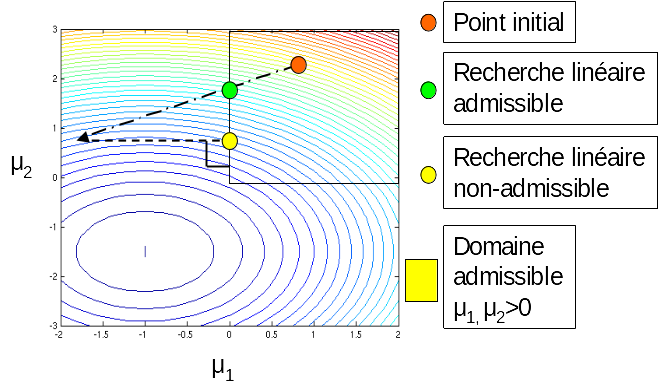
Figure 5.2.4.2-a: variants of linear search.
Here is the linear search algorithm:
\(\mathit{RechLine}\) |
||
\(\mathit{Ini}\) |
Contact status \(\left[{A}^{\text{c}}\right]\leftarrow \left[{A}_{k}^{\text{c}}\right]\) and \({\Xi }^{\text{c}}\leftarrow {\Xi }_{k}^{\text{c}}\) |
|
Calculation of the second limb \(\left\{F\right\}\mathrm{=}{\left[{A}^{\text{c}}\right]}^{T}\mathrm{.}\left\{Z\right\}\) |
||
\(\left[K\right]\mathrm{.}\left\{\delta a\right\}\mathrm{=}\left\{F\right\}\to \left\{\delta a\right\}\) resolution |
||
Calculation of \(\alpha \mathrm{=}\frac{\langle r\rangle \mathrm{.}\left\{{r}^{p}\right\}}{\langle \delta a\rangle \mathrm{.}\left\{F\right\}}\) |
||
If ADMISSIBLE |
||
\(\mathrm{\forall }J\mathrm{\in }{\Xi }^{\text{l}}\mathrm{:}\text{Si}{\left\{Z\right\}}_{J}<0\text{alors}\alpha \mathrm{=}\underset{J\mathrm{\in }{\Xi }^{\text{l}}}{\text{min}}(\alpha ,\mathrm{-}\frac{{\left\{{\mu }^{\text{c}}\right\}}_{J}}{{\left\{Z\right\}}_{J}})\) |
||
\(\left\{{\mu }_{k+1}^{\text{c}}\right\}\mathrm{=}\left\{{\mu }_{k}^{\text{c}}\right\}+\alpha \mathrm{.}\left\{Z\right\}\) |
||
\(\left\{\delta {u}_{k+1}\right\}\mathrm{=}\left\{\delta {u}_{k}\right\}\mathrm{-}\alpha \mathrm{.}\left\{\delta a\right\}\) |
||
Sinon |
||
\(\left\{{\mu }_{k+1}^{\text{c}}\right\}\mathrm{=}\left\{{\mu }_{k}^{\text{c}}\right\}+\alpha \mathrm{.}\left\{Z\right\}\) |
||
\(\left\{{\mu }_{k+1}^{\text{c}}\right\}\leftarrow \text{max}(\left\{{\mu }_{k+1}^{\text{c}}\right\},0)\) |
||
Calculation of the second limb \(\left\{F\right\}\mathrm{=}{\left[{A}^{\text{c}}\right]}^{T}\mathrm{.}\left\{{\mu }^{\text{c}}\right\}\) |
||
\(\left[K\right]\mathrm{.}\left\{\delta a\right\}\mathrm{=}\left\{F\right\}\to \left\{\delta a\right\}\) resolution |
||
\(\left\{\delta {u}_{k+1}\right\}\mathrm{=}\left\{\delta {\tilde{u}}^{n}\right\}\mathrm{-}\left\{\delta a\right\}\) |
||
\(F\) |
FIN |
|
At the output of this algorithm, we will have the displacement and the Lagrange multipliers after calculating the progress step: \(\left\{\left\{\delta {u}_{k+1}\right\},\left\{{\mu }_{k+1}^{\text{c}}\right\}\right\}\mathrm{=}\mathit{RechLine}(\left\{Z\right\},\left\{r\right\},\left\{{r}^{p}\right\})\). This algorithm includes two resolutions but using the matrix \(\left[K\right]\) already factored (it is the global matrix of the balance problem), we therefore only do a downhill ascent, which is inexpensive.
The inadmissible variant is forced to recalculate a displacement increment compatible with the positivity constraint on the contact multipliers.
5.2.4.3. Pre-conditioning#
In the GCP algorithm, there is mention of an optional call to a preconditioner. The aim of this preconditioner is to accelerate the convergence of the method. Its definition comes from the following functional analysis considerations: in the update phase \(\left\{{\mu }_{k+1}^{\text{c}}\right\}\mathrm{=}\left\{{\mu }_{k}^{\text{c}}\right\}+\alpha \mathrm{.}\left\{{Z}_{k}\right\}\) and if the preconditioner has not been used, the field \(\left\{{\mu }_{k}^{\text{c}}\right\}\) belongs to \({H}^{-1/2}({\Gamma }_{\text{c}})\) while \(\left\{{Z}_{k}\right\}\) belongs to \({H}^{1/2}({\Gamma }_{\text{c}})\). So this sum does not make mathematical sense. To give it one, you have to send \(\left\{{Z}_{k}\right\}\) in \({H}^{-1/2}({\Gamma }_{\text{c}})\), this is the preconditioning operation. Knowing that \(\left\{{Z}_{k}\right\}\) is obtained by the expression \(\left\{{Z}_{k}\right\}\mathrm{=}\left\{{r}_{k}^{p}\right\}+{\gamma }_{k}\mathrm{.}\left\{{Z}_{k\mathrm{-}1}\right\}\), it is on \(\left\{{r}_{k}^{p}\right\}\) that we will operate. This is what the preconditioner does by solving the following auxiliary problem:
We therefore solve a displacement problem imposed on the part where the contact is effective and we recover the reactions to embedding \(\left\{{r}_{k}^{p}\right\}\) that belong to \({H}^{-1/2}({\Gamma }_{\text{c}})\). In domain decomposition terminology, this is a Dirichlet preconditioner.
To solve this auxiliary problem, a conjugate gradient algorithm is also used, but without projection because no positivity constraints appear there. This iterative approach allows for an approximate resolution in order to save computation time.
\(\left\{X\right\}\) the research direction;
\(\left\{s\right\}\) the sub-gradient.
Here is the pre-conditioner algorithm:
\(\mathit{PreCond}\) |
|||
\(\mathit{Ini}\) |
\(\left\{{a}_{0}\right\}\mathrm{=}0\) \(\left[{A}^{\text{c}}\right]\leftarrow \left[{A}_{k}^{\text{c}}\right]\) and \({\Xi }^{\text{c}}\leftarrow {\Xi }_{k}^{\text{c}}\) contact status |
||
If \({\Xi }^{\text{c}}\mathrm{=}\mathrm{\varnothing }\) |
|||
Goto Fin \(F\) |
|||
\({B}_{p}\) |
Loop on \(p\mathrm{=}\mathrm{1,}{\mathit{Iter}}_{\mathit{max}}\) |
||
Calculating the gradient \(\left\{{s}_{p}\right\}\mathrm{=}\left[{A}^{\text{c}}\right]\mathrm{.}\left\{{a}_{p\mathrm{-}1}\right\}\mathrm{-}\left\{r\right\}\) |
|||
Residue calculation \(\varepsilon \mathrm{=}\underset{J\mathrm{\in }{\Xi }^{\text{c}}}{\mathit{max}}\left\{{s}_{p}\right\}\) |
|||
If \(\varepsilon <{\varepsilon }_{\mathit{precond}}\) |
|||
Goto Fin \(F\) |
|||
If \(p\mathrm{=}1\) or update |
|||
\(\left\{{X}_{p}\right\}\mathrm{=}\left\{{s}_{p}\right\}\) |
|||
Otherwise, conjugation |
|||
\(\beta \mathrm{=}\frac{\langle {s}_{p}\rangle \mathrm{.}\left\{{s}_{p}\right\}}{\langle {s}_{p\mathrm{-}1}\rangle \mathrm{.}\left\{{s}_{p\mathrm{-}1}\right\}}\) |
|||
\(\left\{{X}_{p}\right\}\mathrm{=}\left\{{s}_{p}\right\}+\beta \mathrm{.}\left\{{X}_{p\mathrm{-}1}\right\}\) |
|||
Calculation of the second limb \(\left\{F\right\}\mathrm{=}{⌊{\left[{A}^{\text{c}}\right]}^{T}\mathrm{.}\left\{{X}_{p}\right\}⌋}_{{\Xi }^{\text{c}}}\) |
|||
\(\left[K\right]\mathrm{.}\left\{\delta a\right\}\mathrm{=}\left\{F\right\}\to \left\{\delta a\right\}\) resolution |
|||
Calculating Schur’s complement \({\left\{\delta a\right\}}_{\text{schur}}\mathrm{=}{⌊\left[{A}^{\text{c}}\right]\mathrm{.}\left\{\delta a\right\}⌋}_{{\Xi }^{\text{c}}}\) |
|||
Calculating the progress step \(\alpha \mathrm{=}\frac{\langle {s}_{p}\rangle \mathrm{.}\left\{{s}_{p}\right\}}{\langle F\rangle \mathrm{.}{\left\{\delta a\right\}}_{\text{schur}}}\) |
|||
New sub-gradient \(\left\{{s}_{p}\right\}\mathrm{=}\left\{{s}_{p\mathrm{-}1}\right\}+\alpha \mathrm{.}\left\{{X}_{p}\right\}\) |
|||
New trip \(\left\{{a}_{p}\right\}\mathrm{=}\left\{{a}_{p\mathrm{-}1}\right\}\mathrm{-}\alpha \mathrm{.}\left\{\delta a\right\}\) |
|||
\({B}_{k}\) |
End Loop \(k\mathrm{=}k+1\) |
||
\(F\) |
FIN |
||
\(\left\{{r}_{k}^{p}\right\}\mathrm{=}\left\{{s}_{p}\right\}\) Projection: \(({\mathit{max}}_{J}({r}_{k}^{p}\mathrm{,0})\mathit{si}{\mu }_{J}<0)\) |
|||
At the output of this algorithm, we will have pre-conditioned sub-gradient: \(\left\{{r}_{k}^{p}\right\}\mathrm{=}\mathit{PreCond}(\left\{{r}_{k}\right\})\).
5.2.4.4. Algorithm#
Here is the overall algorithm for method GCP:
\(\mathit{Ini}\) |
if:math: langle {mu} _ {imathrm {-} 1}} ^ {text {c}}ranglemathrm {cdot}left{{mu} _ {imathrm {-}} _ {imathrm {-}} 1} ^ {text {-} 1}} ^ {text {c}}}ranglemathrm {cdot}left{{mu}} _ {imathrm {-}} _ {imathrm {-} 1}} ^ {text {c}}}right}mathrm {ne} 0 then:math:` mathrm {[} Kmathrm {]}mathrm {.} left{vright}mathrm {=}}mathrm {[} {A} _ {imathrm {-} 1} ^ {text {c}}} {mathrm {]}} {mathrm {]}}}} ^ {T}mathrm {.} left{{mu} _ {imathrm {-} 1}} ^ {text {c}}right}toleft{vright} si:Math:langle {mu}} _ {imathrm {-} 1} ^ {text {c}}ranglemathrm {cdot}left{mu} _ {imathrm {-} 1}} ^ {text {c}}ranglemathrm {cdot}left{mu} _ {imathrm {-} 1}} ^ {text {c}} {text {c}}}right}mathrm {=} 0` then:math: left{vright}}mathrm {=}mathrm {=} =}left\ left{0right}}}left{0right}}left{0right}} Calculation of:math: {mathit {delta u}}} _ {0} ^ {n} =mathrm {=} =}leftleft{0right} =left{0right} =left{0right}} =left{0right}} =delta {ackrel {} {u}}} ^ {n} -v | Rating of:math: {Xi} _ {0} _ {0} ^ {text {c}} {text {c}}}mathrm {=}left{in} {xi} ^ {text {l}}}mathrm {mid}} ^ {text {c}} ^ {text {c}, n} {text {l}} ^ {text {l}}} ^ {text {l}}} ^ {text {l}}} ^ {text {l}}} ^ {text {l}}} ^ {text {l}}} ^ {text {l}}} ^ {text {l}}} ^ {text {l}}} ^ {text {l}}} ^ {text {J} <0right} | |
||
\({B}_{k}\) |
Loop on \(k\mathrm{=}\mathrm{1,}{\mathit{Iter}}_{\mathit{max}}\) |
||
\({\Xi }_{k}^{\text{c}}\leftarrow {\Xi }_{k\mathrm{-}1}^{\text{c}}\) |
|||
Calculating the sub-gradient \(\left\{{r}_{k}\right\}\mathrm{=}(\left[{A}_{k}^{\text{c}}\right]\mathrm{.}\left\{\delta {u}_{k\mathrm{-}1}^{n}\right\}\mathrm{-}\left\{{d}^{\text{c},n\mathrm{-}1}\right\})\) |
|||
Sub Gradient Projection \(\left\{{r}_{k}\right\}\mathrm{=}\underset{J\mathrm{\in }{\Xi }^{\text{l}}}{\mathit{max}}(\left\{{r}_{k}\right\},0)\) |
|||
Residue calculation \(\varepsilon \mathrm{=}\underset{J\mathrm{\in }{\Xi }^{\text{l}}}{\mathit{max}}\left\{{r}_{k}\right\}\) |
|||
Preconditioning \(\left\{{r}_{k}^{p}\right\}\mathrm{=}\mathit{PreCond}(\left\{{r}_{k}\right\})\) |
|||
Conjugation |
|||
Calculating the coefficient \({\gamma }^{k}\mathrm{=}\frac{\langle {r}_{k}\rangle \mathrm{.}\left\{{r}_{k}^{p}\right\}\mathrm{-}\langle {r}_{k}\rangle \mathrm{.}\left\{{r}_{k\mathrm{-}1}^{p}\right\}}{\langle {r}_{k\mathrm{-}1}\rangle \mathrm{.}\left\{{r}_{k\mathrm{-}1}^{p}\right\}}\) |
|||
\(\left\{{Z}_{k}\right\}\mathrm{=}\left\{{r}_{k}\right\}+{\gamma }^{k}\mathrm{.}\left\{{Z}_{k\mathrm{-}1}\right\}\) |
|||
Linear Search \(\left\{\left\{\delta {u}_{k+1}\right\},\left\{{\mu }^{\text{c}}\right\}\right\}\mathrm{=}\mathit{RechLine}(\left\{Z\right\},\left\{r\right\},\left\{{r}^{p}\right\})\) |
|||
\({B}_{k}\) |
Buckle \(k\mathrm{=}k+1\) |
||
\(F\) |
FIN |
||
The following comments can be made about the algorithm:
During the linear search, the resolution of the \(\left[K\right]\mathrm{.}\left\{\mathrm{\delta }a\right\}={\left[{A}^{\text{c}}\right]}^{T}\mathrm{.}\left\{Z\right\}\) system and the calculation of the term \(\langle \delta a\rangle \mathrm{.}{\left[{A}^{\text{c}}\right]}^{T}\mathrm{.}\left\{Z\right\}\), we perceive that the algorithm presented is the iterative version of the active constraints method. In fact, if you explain the term \(\langle \delta a\rangle \mathrm{.}{\left[{A}^{\text{c}}\right]}^{T}\mathrm{.}\left\{Z\right\}\), you get \(\langle Z\rangle \mathrm{.}(\left[{A}_{\text{c}}\right]\mathrm{.}{\left[K\right]}^{\mathrm{-}1}\mathrm{.}{\left[{A}_{\text{c}}\right]}^{T})\mathrm{.}\left\{Z\right\}\). We find the Schur complement \({\left[K\right]}_{\text{schur}}\mathrm{=}\left[{A}^{\text{c}}\right]\mathrm{.}{\left[K\right]}^{\mathrm{-}1}\mathrm{.}{\left[{A}^{\text{c}}\right]}^{T}\) which is explicitly built in the active constraints method. As in all iterative methods, the Projected Conjugate Gradient does not build this operator but uses its effect on a vector (here on \(\left\{Z\right\}\));
To be really effective, this algorithm must be used with a direct solver or an iterative solver preconditioned by the LDLT_SP method.
With a direct solver, the system matrix being already factored, each resolution comes down to a downhill ascent:
With an iterative solver preconditioned by the LDLT_SP method, each resolution comes down to a few iterations of the iterative solver.
We combine at each iteration.
5.3. The penalized method in contact — ALGO_CONT =” PENALISATION “#
The penalized method is particularly appropriate when the \(\left[K\right]\) matrix is not symmetric. However, it requires a study of sensitivity to the penalty coefficient (of the dimension of a relationship of a force by a displacement) and at least a verification of the results that the contact is correctly taken into account (the structures do not interpenetrate each other).
5.3.1. Balance of the structure in the presence of contact#
Recall that the equilibrium equation in the presence of contact is written as:
In the case of penalized contact, the contact force is written as:
: label: eq-138
left{{L} _ {i} ^ {text {c}} {text {c}}right}right}mathrm {=} {left{{L} _ {i} ^ {text {c}, n}right} ^ {text {c}} ^ {text {c}, n}rightright}}}rightright}}rightright}}rightright}}rightright}}rightright}}rightright}}rightrightmathrm {[} {A} ^ {text {c}} {mathrm {]}}} ^ {T}mathrm {.} (left [{A} ^ {text {c}}}right]mathrm {.} left{delta {u} ^ {n}right} {n}right}mathrm {-}left{{d} ^ {text {c}, nmathrm {-} 1}right})
After linearization of the equilibrium equation (), we introduce the tangent matrix \(\left[{K}^{\text{m},n\mathrm{-}1}\right]\) which will contain the contributions resulting from the linearization of internal and external forces and the matrix \(\left[{K}^{\text{c},n\mathrm{-}1}\right]\) for contact forces:
The second member is equal to:
Regarding the algorithm, we saw in § 4.3.6.2 that it acts to correct the non-contact balance problem.
When we’re in the contact algorithm, at Newton iteration \(n\), we’re evaluating \(\left[{K}_{i}^{\text{c},n+1}\right]\) and \(\left\{{L}_{i}^{\text{c},n}\right\}\), which won’t be used until the next Newton iteration. There is a time lag of one iteration: you necessarily need at least two Newton iterations to solve a problem with penalized contact.
5.3.2. Algorithm#
\(\mathit{Ini}\) |
Calculating \({⌊\left\{{\tilde{d}}^{\text{c},n}\right\}⌋}_{{\Xi }^{\text{l}}}\) |
Evaluating \({\Xi }^{\text{c}}\mathrm{=}\left\{J\mathrm{\in }{\Xi }^{\text{l}}\mathrm{\mid }{⌊\left\{{\tilde{d}}^{\text{c},n}\right\}⌋}_{J}<0\right\}\) and \(\left[{A}^{\text{c},n}\right]\) |
|
Contact pressures \({⌊\left\{{\mu }^{\text{c},n}\right\}⌋}_{{\Xi }^{\text{c}}}\mathrm{=}\mathrm{-}{E}_{N}\mathrm{.}{⌊\left\{{\tilde{d}}^{\text{c},n}\right\}⌋}_{{\Xi }^{\text{c}}}\) |
|
Second member \(\left\{{L}_{i}^{\text{c},n}\right\}\mathrm{=}{\left[{A}^{\text{c},n}\right]}^{T}\mathrm{.}{⌊\left\{{\mu }^{\text{c},n}\right\}⌋}_{{\Xi }^{\text{c}}}\) |
|
Matrix \(\left[{K}^{\text{c},n+1}\right]\mathrm{=}{E}_{N}\mathrm{.}{\left[{A}^{\text{c},n}\right]}^{T}\mathrm{.}\left[{A}^{\text{c},n}\right]\) |
Notes:
Quantities \(\left[{K}_{i}^{\text{c}}\right]\) and \(\left\{{L}_{i}^{\text{c}}\right\}\) are only evaluated for active bonds. For the rest of the unknowns, we initialize to zero;
The change in the system does not introduce any new variables in relation to the non-contact problem;
There is no \(k\) clue in the various quantities (in particular the set of active links or the contact matrix) because it is not an iterative algorithm;
To calculate the matrix, we proceed in two stages: evaluations of the elementary matrices, then assembly. But these two operations are specific to discrete contact, we do not use the generic elemental calculations/assembly mechanism of Code_Aster.
The choice of the penalty coefficient is crucial: too low, interpenetrations will be observed, too strong, the conditioning of the tangent matrix is deteriorating.