2. Contact and friction mechanics#

2.1. Problem definition and ratings#

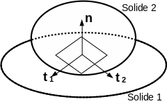
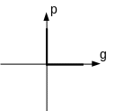
We consider two solids that can come into contact by friction; the contact zone is either point, linear, or surface. Let \(\left\{n\right\}\) be the outgoing normal at the surface of one of the solids in contact and \(\left\{u\right\}\) the displacement vector between the two solids. So \(g\mathrm{=}\langle u\rangle \mathrm{.}\left\{n\right\}\) is the displacement projected on this normal, we’ll call it game. From the data of the Cauchy constraint, we define the pressure [1] _ \(p\mathrm{=}\langle n\rangle \mathrm{.}\left[\sigma \right]\mathrm{.}\left\{n\right\}\) and the tangential shear stress \(\left\{r\right\}\mathrm{=}\left[\sigma \right]\mathrm{.}\left\{n\right\}\mathrm{-}p\mathrm{.}\left\{n\right\}\) as being exerted by one of the surfaces on the other.

Figure 2.1-a : definition of the local contact coordinate system.

The direction of the shear force in the contact zone is a vector \(\left\{t\right\}\) located in the tangential plane \((\left\{{t}_{1}\right\},\left\{{t}_{2}\right\})\) shown in figure (). Equation () defines the shear stress \(r\) exerted by the solid (2) on the solid (1) per unit contact area.

(2.1)#\[ \begin{align}\begin{aligned} \ left\ {r\ right\}\ mathrm {=}\ left [\ sigma\ right]\ mathrm {.} \ left\ {n\ right\}\ mathrm {-} (\ langle n\ rangle\ mathrm {.} \ left [\ sigma\ right]\ mathrm {.} \ left\ {n\ right\})\ mathrm {.} \ left\ {n\ right\}\ mathrm {=} r\ mathrm {.} \ left\ {t\ right\}\\ \ textrm {with}\\ r\ mathrm {=}\ mathrm {\ parallel}\ left\ {r\ right\}\ mathrm {\ parallel}\end{aligned}\end{align} \]

2.2. Signorini contact conditions#

The two variables defining contact have been introduced:

The signed distance between the two surfaces or « gap » :math:`g`; *

Contact pressure \(p\);

The three Hertz-Signorini-Moreau contact conditions are then defined

Geometric condition: impenetrability of matter (Signorini-Hertz).

(2.2)#\[\begin{split} g\ ge 0\ iff\ {\ begin {array} {array} {c} g>0\ text {no contact}\\ g=0\ text {contact}\ end {array}\end{split}\]

Mechanical condition: intensity (Signorini-Hertz)

(2.3)#\[\begin{split} p\ mathrm {\ ge} 0\ mathrm {\ iff}\ mathrm {\ {}\ begin {array} {c} p>0\ text {contact}\\ p\ mathrm {=} {=} 0\ text {no contact}\ end {array}\end{split}\]

Energy condition: complementarity/exclusion (Moreau)

\[\]

: label: eq-4

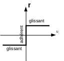
ptext {.} g=0iff{begin {array} {c} p=0text {detachment}\ g=0text {contact}text {contact}end {array}

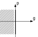
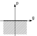
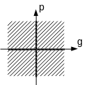
Graphically, the three conditions are represented in figure () where the shaded areas represent the excluded areas and the white areas or black lines represent the authorized areas.




Impenetrability	Intensity	Complementarity
Figure 2.2-a : graphical representation of Hertz-Signorini-Moreau conditions.

By combining the three conditions we obtain the graph in figure ().

Figure 2.2-b : graph of the unilateral contact condition.

The contact problem thus posed introduces a non-univocal relationship (\(p\) is not a function of \(g\)), semi-definite positive and non-differentiable relationship in \(p=g=0\). This is a mathematically difficult problem to deal with. Contact is a reversible and conservative phenomenon for which an energy potential can be introduced and whose result does not depend on the loading path; it is similar to Hencky’s elastoplastic model. Signorin’s law of contact is written as:

\[\]

: label: eq-5

mathrm {{}begin {array} {cc} {cc} gmathrm {ge} 0& (a)\ pmathrm {ge} 0& (b)\ pmathrm {.} gmathrm {.} gmathrm {=} 0& (c)end {array}

Notes:

The contact is assumed to be non-adherent thanks to the second condition (intensity).
The third condition allows the unilateral contact problem to be well posed in order to be solved by classical optimization techniques under constraints (introduction of Kuhn & Tucker conditions) such as the active constraints method.

2.3. Formulation of the friction problem#

2.3.1. Definitions#

The friction criteria chosen are of the form:

(2.4)#\[ h (\ left\ {r\ right\})\ mathrm {\ le} 0\]

where \(h(\left\{r\right\})\) is a convex function. The non-slip domain is defined by the inside of the convex. Two friction criteria of the form \(h(\left\{r\right\})\mathrm{\le }0\) are particularly used: the Tresca criterion and the Coulomb criterion.

2.3.2. The Tresca criterion#

The Tresca criterion is defined by the following function \(h(\left\{r\right\})\):

(2.5)#\[ \begin{align}\begin{aligned} h (\ left\ {r\ right\})\ mathrm {=}\ mathrm {=}\ mathrm {\ parallel}\ mathrm {\ parallel}\ mathrm {-} k\ mathrm {-} k\ mathrm {\ the} 0\\ \ textrm {with :math:`k` a given constant}\end{aligned}\end{align} \]

Note \(C\) the convex disk with radius \(k\) centered at the origin defined by:

(2.6)#\[ C\ mathrm {=}\ left\ {\ left\ {\ left\ {r\ right\}\ text {such as}\ mathrm {\ parallel}\ left\ {r\ right\}\ mathrm {\ parallel}\ mathrm {\ parallel}\ mathrm {\ le} k\ right\}\]

The non-sliding condition is then defined by the belonging of \(\left\{r\right\}\) to the inside of the disk \(C\). In case of sliding, for \(\left\{r\right\}\) located on the border of \(C\), the sliding direction \(\left\{t\right\}\) of \(\left\{\dot{u}\right\}\) is given by the normal to the criterion in \(\left\{r\right\}\), as shown on the.

Figure 2.3.2-a : friction disk for the Tresca criterion.

This results in an expression for the sliding speed analogous to the plastic multiplier:

(2.7)#\[ {\ dot {u}} _ {t} =\ lambda\ mathrm {.} r\]

With \(\lambda \mathrm{\ge }0\), that is, the sliding speed is in the same direction as the tangential stress.

2.3.3. The Coulomb criterion#

The Coulomb criterion is defined by the following function \(h(\left\{r\right\})\):

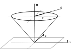
(2.8)#\[ \begin{align}\begin{aligned} h (\ left\ {r\ right\},\ mu, p)\ mathrm {=}\ mathrm {\ parallel}\ left\ {r\ right\}\ mathrm {\ parallel}\ mathrm {\ parallel}\ mathrm {-} k (\ mu, p)\ mathrm {\ the} 0\\ \ textrm {and}\\ k\ mathrm {=}\ mu\ mathrm {.} \ mathrm {\ mid} p\ mathrm {\ mid}\end{aligned}\end{align} \]

The value of \(k\) depends on the contact pressure \(p\) and the Coulomb friction coefficient \(\mu\) Thus defined, \(h\) is a cone. In case of sliding, for \(\left\{r\right\}\) located on the border of \(h\), the sliding direction \(\left\{t\right\}\) of \(\dot{u}\) is not given by the normal to the criterion in \(\left\{r\right\}\), but by the normal to the convex disk \(C\) of radius \(k\mathrm{=}\mu \mathrm{.}\mathrm{\mid }p\mathrm{\mid }\). The Tresca criterion corresponds to a « slice » along the plane orthogonal to the Coulomb cone.

Figure 2.3.3-a : cone of friction for the Coulomb criterion.

2.3.4. Application to Coulomb friction#

Let us write the system of equations and inequalities that must be verified by these quantities in the case of the Coulomb friction criterion:

(2.9)#\[\begin{split} \ mathrm {\ {}\ begin {array} {cc} {cc} g\ mathrm {\ ge} 0& (a)\\ p\ mathrm {\ ge} 0& (b)\\ p\ mathrm {.}.} g\ mathrm {{cc} g\ mathrm {=} 0& (c)\\ mathrm {\ parallel}\ left\ {r\ right\}\ mathrm {\ right\}}\ mathrm {parallel}\ left\ {r\ right\}}\ mathrm {\ right\}\}\ mathrm {-}\ mu\ mathrm {.} \ mathrm {\ mid} p\ mathrm {\ mid}\ mathrm {\ mid}\\ mid}\\\ left\ {\ dot {u}} _ {t}\ right\}\ right\}\ right\}\ right\}\ right\}\ right\}\ mathrm {}\ mathrm {}\ mathrm {=}\ lambda\ mathrm {.} \ left\ {r\ right\} & (e)\\\ lambda\ mathrm {.} (\ mathrm {\ parallel}\ left\ {r\ right\}\ mathrm {\ parallel}\ mathrm {-}\ mu\ mathrm {.} \ mathrm {\ mid} p\ mathrm {\ mid})\ mathrm {\ mid})\ mathrm {\ mid})\ mathrm {\ ge} 0& (g)\ end {array}\end{split}\]

The first set of equations and inequalities (a-c) corresponds to contact management. The second batch (d-g) corresponds to the description of friction obeying the Coulomb criterion. It involves several fields and links them together: the normal pressure \(p\), the shear stress \(\left\{r\right\}\) and the tangent speed \(\left\{{\dot{u}}_{t}\right\}\). It can be understood as follows:

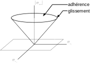
(2.10)#\[\begin{split} \ mathrm {\ {}\ begin {array} {cc} {cc}\ text {If}\ mathrm {\ parallel}\ left\ {r\ right\}\ mathrm {\ parallel}} <\ mu\ mathrm {.} \ mathrm {\ mid} p\ mathrm {\ mid}\ text {\ mid}\ text {then}\ lambda\ mathrm {=} 0\ text {and}\ left\ {{\ dot {u}}} _ {t}\\\\\\\\\\\ dot {u}}} _ {t}\\ right\ right\}\ right\}\ right\}\ mathrm {\ parallel}\ mathrm {=}\ mu\ mathrm {.} \ mathrm {\ mid} p\ mathrm {\ mid}\ text {then}\ lambda >0\ text {and}\ left\ {\ dot {u}} _ {t}\ right\}\ right\}\ right\}\ right\}\ right\}\ right\}\ right\ right\}\ right\}\ mathrm {}\ mathrm {=}\ lambda\ mathrm {.} \ left\ {r\ right\} & (b)\ end {array}\end{split}\]

Figure () shows the Coulomb cone. In the stress space, the friction contact force can only be found inside the Coulomb cone: if it is strictly inside, the contact is adherent; if it is on the surface of the cone, the contact is slippery.

Figure 2.3.4-a : interpretation of the friction cone.

Another representation of this criterion can be given (see figure ()).

Figure 2.3.4-b : Coulomb friction graph.

Friction induces the concept of threshold. The relationship introduced by Coulomb friction is a non-univocal and non-differentiable relationship. Unlike contact, the relationship is not associative [2] _ and cannot derive directly from an energy dissipation potential. It will also be noted that friction links the relative speed of the two surfaces and not the displacement. However, we can establish that in statics, if we solve the problem in incremental form (which is the case when using Newton as in Code_Aster), we can replace the relative speed by the tangential displacement increment.

2.4. Formulation by differential inclusions#

The non-differentiable nature of friction relationships leads us to introduce the concept of differential sub-inclusion.

Note \(V\) the set of kinematically admissible movements of the problem. The relationship between the relative sliding speed \(\left\{\dot{u}\right\}\) and the shear stress \(r\) reflects the two possible states of the system: non-slip or relative sliding in the normal direction in \(\left\{r\right\}\) to the convex disk \(C\). For the three criteria presented, the function \(\left\{{\dot{u}}_{t}\right\}(r)\) and its inverse \(\left\{r({\dot{u}}_{t})\right\}\) both belong to the sub-differentials of two conjugated pseudopotentials \({\Psi }_{c}(r)\) and \({\Psi }_{c}^{\text{*}}({\dot{u}}_{t})\), so that we can write:

(2.11)#\[ \begin{align}\begin{aligned} \ left\ {\ dot {u}\ right\}\ right\}\ mathrm {\ in}\ mathrm {\ partial} {\ psi}} _ {c} (r)\\ \ textrm {and}\\ \ left\ {r\ right\}\ mathrm {\ in}\ mathrm {\ in}\ mathrm {\ partial} {\ Psi} _ {c} ^ {\ text {*}}} (\ dot {u})\end{aligned}\end{align} \]

The appearance of differential inclusions comes from the non-differentiable nature of the laws of touch-friction. In fact, \({\Psi }_{c}\) designates the indicative function of the convex disk \(C\) with radius \(k\), centered at the origin, previously defined. It is such that:

(2.12)#\[\begin{split} {\ Psi} _ {c} (r)\ mathrm {=}\ mathrm {=}\ mathrm {\ {}\ begin {array} {c} 0\ text {si}\ left\ {r\ right\}\ mathrm {\ right\}}\ mathrm {\ in}}\ mathrm {\ in}}\ mathrm {\ in} C\\ +\ mathrm {\ infty}\ text {otherwise}\ end {array}\end{split}\]

The \(\partial {\Psi }_{c}(r)\) subdifferential of the \({\Psi }_{c}\) function in \(r\) merges with the external normal at \(C\) in \(\left\{r\right\}\). \({\Psi }_{c}^{\text{*}}(\dot{u})\mathrm{=}k\mathrm{\parallel }\dot{u}\mathrm{\parallel }\), where \(k\) is the frictional resistance threshold, \({\mathrm{\Psi }}_{c}^{\text{*}}\) is the Fenchel conjugate of the indicator function \({\mathrm{\Psi }}_{c}\). \({\mathrm{\Psi }}_{c}^{\text{*}}\) is positively homogeneous of degree one. This function is interpreted as the density of power dissipated in the sliding. Using the notions of subdifferential, we can establish the following relationships for \(\left\{\dot{u}\right\}\) and \(\left\{r\right\}\) associates:

(2.13)#\[\begin{split} \ mathrm {\ {}\ begin {array} {c} {c}\ dot {u}\ dot {u}\ mathrm {\ in}\ mathrm {\ partial} {\ Psi} _ {c} (r)\ mathrm {\ iff}\ mathrm {\ iff}\\\\\\\\\\ dot {u}\ mathrm {.} (r\ text {'}\ mathrm {-} r)\ mathrm {\ le} 0,\ mathrm {\ forall} r\ text {'}\ mathrm {\ in} C\ end {array}\\ end {array}\\\ array}\\\ r\ mathrm {\ mathrm {\ le}} 0,\ mathrm {\ le} 0,\ mathrm {\ forall} r\ text {\ in}}\ mathrm {\ in}}\ mathrm {\ in}}\ mathrm {\ in}}\ mathrm {\ in}}\ mathrm {\ in}}\ mathrm {\ in}}\ mathrm {\ in}} {\ dot u})\ mathrm {\ iff}\ mathrm {\ {}\ begin {}\ begin {array} {c}\ dot {u}\ mathrm {\ in} V\\ r\ mathrm {.} (\ dot {v}\ mathrm {-}\ dot {u})\ mathrm {\ dot {u})\ mathrm {-}\ dot {v})\ mathrm {-}\ dot {v})\ mathrm {-}\ dot {u})\ mathrm {-}\ dot {v})\ mathrm {-} {\ dot {v})\ mathrm {-} {\ dot {u})\ mathrm {-} {\ dot {v})\ mathrm {-} {\ dot {u})\ mathrm {-}\ dot {u})\ mathrm {-}\ dot {u})\ mathrm {-}\ dot {u})\ mathrm {-}\ dot {v})\ v}\ mathrm {\ in} V\ end {array}\\ {\ array}\\ {array}\\ {array}\\\ array}\\ end {array}\\ end {array}\\ end {array}\\ {\ array}\\ {\ Psi}\ {\ psi} _ {\ psi} _ {c} (r)\ mathrm {\ c} (r)\ mathrm {c} (r)\ mathrm {=} (r)\ mathrm {c} (r)\ mathrm {=} (r)\ mathrm {=} (r)\ mathrm {\ c} (r)\ mathrm {=} (r)\ mathrm {=} (r)\ mathrm {=} (r)\ mathrm\ mathrm {\ parallel}\ end {array}\end{split}\]

Notes:

The two conjugated pseudopotentials presented are non-differentiable.
Once the normal reaction for the Coulomb criterion is known, we come back locally to a Tresca friction criterion whose threshold is as follows: math: k=mumathrm {.} |p|.
The local criteria adopted having a circular form we deduce that \(\dot{u}\mathrm{\in }\mathrm{\partial }{\Psi }_{c}(r)\) implies that there is \(\lambda\) real positive such as \(\dot{u}=\lambda r\).
The formulation of the speed problem suggests an incremental numerical resolution of the friction problem. The resolution of the balance problem will therefore be presented in incremental form.

2.5. Solving the balance problem#

Consider two solids with a total volume \(\mathrm{\Omega }\) whose contact surface is \({\mathrm{\Gamma }}_{c}\). To simplify, the existence of a differentiable deformation energy will be assumed to characterize the response of the two separated solids to external stresses (in fact, it can be demonstrated that the results given below are independent of this hypothesis). Note \(V\) the set of kinematically admissible displacement fields, constrained by compliance with the contact and friction conditions on the interface. The balance of the two solids in the absence of friction is written as:

(2.14)#\[ \begin{align}\begin{aligned} \ textrm {*Find*}\\ U\\ \ textrm {*kinematically admissible field of movement such as*}\\ \ left\ {U=\ underset {v\ in V} {\ text {argmin}}\ left [\ Phi (\ varepsilon (v)) -W (v)\ right]\ right\}\ iff\ left\ {\ iff\ left\ left\ {\ Phi (U) -W (U)\ {\ Phi (U) -W (U)}\ left [\ Phi (v) -W (v)] -W (v)\ right]\ right\}\ iff\ left\ iff\ left\ left\ {\ Phi (U) -W (U) -W (v) -W (v),\ right]\ right\}\ iff\ left\ iff\ left\ left\ {\ Phi (U) -W\end{aligned}\end{align} \]

In elasticity, \(\mathrm{\Phi }(v)={\int }_{\mathrm{\Omega }}\phi (\epsilon (v))\text{.}d\mathrm{\Omega }\) is the deformation energy. The \(W(v)\) function represents the work of external forces. A necessary condition (which becomes sufficient if \(\mathrm{\Phi }\) is strictly convex) for this balance to be verified is that:

(2.15)#\[ D\ mathrm {\ Phi} (U) -\ mathit {DW}\ left (U\ right) =D\ mathrm {\ Phi} (U) - {L} ^ {\ text {ext}} =0\]

where \(D\) is the operator derived from Gâteaux and \({L}^{\text{ext}}\) is the linear form associated with external forces.

With the introduction of friction, the problem should be addressed in incremental form. We are led (see [2] and [3]) to the following minimization problem on all \(\overline{V}\) of the kinematically admissible fields constrained by compliance with the contact and friction conditions on the interface:

(2.16)#\[ \begin{align}\begin{aligned} U\\ \ textrm {*known, find* :math:`\mathrm{\Delta }U\in \overline{V}` *such as*}\\ U+\ Delta U=\ underset {\ Delta v\ in\ stackrel {} {V}} {\ text {argmin}}\ left [\ Phi (\ varepsilon (U+\ Delta v)) + {\ Psi}\ in\ stackrel {} {c}} ^ {\ text {*}}} {\ text {argmin}}}\ left [\ Phi (\ varepsilon (U+\ Delta v))) + {\ Psi}\ in\ in\ in\ stackrel {c}} ^ {\ text {*}}} (\ Delta v)\ right]\end{aligned}\end{align} \]

\(U+\mathrm{\Delta }U\) is thus a solution to:

(2.17)#\[ \ underset {\ Delta v\ mathrm {\ in}\ stackrel {} {V}} {\ text {min}}\ left [\ underset {\ Omega} {\ mathrm {\ int}}}\ varphi (\ varepsilon (\ varepsilon (U+\ Delta v)) d\ omega +\ underset {{\ gamma}} {\ gamma}} {\ mathrm {\ int}}}\ varphi (\ varepsilon (U+\ Delta v)) d\ Omega +\ underset {\ Gamma} _ {c}}} {\ mathrm {\ int}}}\ varphi (\ varepsilon (U+\ Delta v)) d\ Omega +\ underset {\ Gamma}} {\ Gamma} int}} k\ mathrm {\ mid}\ Delta {v}\ Delta {v} _ {t}\ mathrm {\ mid} d {\ Gamma} _ {c}\ mathrm {-} W (U+\ Delta v)\ right]\]

where \(\Delta {v}_{t}\) is the tangential component of the relative displacement increment [3] _ of solid \(2\) compared to solid \(1\) along the contact surface, with the conventions adopted in § 2.3.

Using the relationships \({\Psi }_{c}^{\text{*}}(\Delta {v}_{t})\mathrm{=}k\mathrm{\mid }\Delta {v}_{t}\mathrm{\mid }\) and \({\Psi }_{c}^{\text{*}}(\Delta {v}_{t})\mathrm{\ge }r\Delta v\) if \(r\in C\) we deduce that \(U+\Delta U\) is the solution of the following \(\text{minmax}\) problem, on the space \(V\) of kinematically admissible fields:

\[\]

: label: eq-20

underset {Delta vin V} {text {Min}} {text {Min}}underset {r} {text {Max}}text {} J (U+Delta v, r)

where functional \(J\) is equal to:

\[\]

: label: eq-21

J (U+Delta v, r) =underset {omega} {omega} {omega} {omega} {omega} {omega} {omega +underset {Gamma} _ {c}}} {int} (rtext {.}) {text {.} Delta {v} _ {t} - {Psi} _ {Psi} _ {c} (r))text {.} d {Gamma} _ {c} -W (U+Delta v)

The presence of the indicator function in this expression indicates that shear \(r\) on the contact surface \({\mathrm{\Gamma }}_{c}\) belongs to the convex friction disk \(C\).

2.6. Variational formulation#

If \(\phi\) is convex, the \(\text{minmax}\) problem to be solved is equivalently in the form:

(2.18)#\[ \begin{align}\begin{aligned} \ textrm {*Find*}\\ \ Delta U\ in V\\ \ textrm {*and* :math:`r\in C` *, a set of independent variables such as*}\\ \ delta J (U+\ Delta U, r)\ni 0\end{aligned}\end{align} \]

This is equivalent to solving the following system of equations at equilibrium:

(2.19)#\[\begin{split} \ mathrm {\ {}\ begin {array} {cc} {cc}\ underset {\ omega} {\ mathrm {\ int}}\ frac {\ mathrm {\ partial}\ varphi} {\ mathrm {\ partial} {\ partial}\ partial}\ varepsilon} (\ varepsilon} (\ varepsilon (U+\ Delta U))\ mathrm {.} \ delta\ varepsilon\ mathrm {.} d\ omega +\ underset {{\ Gamma} _ {c}} {\ mathrm {\ int}}} r\ mathrm {.} \ delta {v} _ {t}\ mathrm {.} d {\ Gamma} _ {c}\ mathrm {-} {L} ^ {\ text {ext}}}\ text {ext}}\ text {.} \ delta v\ mathrm {=} 0& (a)\\\ underset {{\ Gamma} _ {c}} {\ mathrm {\ int}}} (\ delta r\ text {.} \ Delta {U} _ {t}\ mathrm {.} d {\ Gamma} _ {c}\ mathrm {-}\ mathrm {\ partial} {\ Psi} _ {c} (r))\ mathrm {.} (r))\ mathrm {\ Gamma} _ {.} (r))\ mathrm {\ gamma} _ {c} (r))\ mathrm {r)))\ mathrm {\ni} 0& (b)\ end {array}\end{split}\]

or in an equivalent manner:

(2.20)#\[\begin{split} \ mathrm {\ {}\ begin {array} {cc} {cc}\ underset {\ omega} {\ mathrm {\ int}}\ frac {\ mathrm {\ partial}\ varphi} {\ mathrm {\ partial} {\ partial}\ partial}\ varepsilon} (\ varepsilon} (\ varepsilon (U+\ Delta U))\ mathrm {.} \ delta\ varepsilon\ mathrm {.} d\ omega +\ underset {{\ Gamma} _ {c}} {\ mathrm {\ int}}} r\ mathrm {.} \ delta {v} _ {t}\ mathrm {.} d {\ Gamma} _ {c}\ mathrm {-} {L} ^ {\ text {ext}}}\ text {ext}}\ text {.} \ delta v\ mathrm {=} 0& (a)\\\ Delta {U} _ {t}\ mathrm {\ in}\ mathrm {\ partial} {\ Psi} _ {c} (r) & (b) & (b)\\ r\ mathrm {r) & (b)\\ r\ r) & (b)\\ r\ mathrm {.} (r) & (b)\\ r\ mathrm {=} {=} ({\ sigma} _ {1}\ mathrm {.} n)\ mathrm {.} n)\ mathrm {.} (r) & (b)\\ r\ mathrm {.} (r) & (b)\\ r\ mathrm {.} (r) & (b) {on} {\ Gamma} _ {c} & (c)\ end {array}\end{split}\]

As in the previous section, \({L}^{\text{ext}}\) is the linear form associated with external forces. The linear shape \({L}^{\text{frot}}\) is associated with the shear forces exerted by solid \(2\) on the contact surface of solid \(1\). It should also be noted that the variational formulation makes it possible to find not only the equilibrium equations of the system but also the belonging of \(\mathrm{\Delta }{U}_{t}\) to the sub-differential of \({\mathrm{\Psi }}_{c}\).

2.7. Steps for solving the touch-friction problem#

The discrete resolution method implemented in Code_Aster is based on writing interpenetrating relationships on the nodes of the meshes facing each other, which implies:

A discreet description of the contact surfaces (mesh);
The search for the minimum projection distance and the position of this projection (so-called matching operation);
Writing kinematic relationships between nodes;
Algorithms for solving the touch/friction problem;

We will detail each of these aspects later in this document.

For so-called « discrete » formulations (as opposed to the so-called « continuous » formulation, see [R5.03.52]), Code_Aster solves the contact problem by methods that belong to the family of methods called « status method » in the literature, with global-local decoupling.

The touch/friction algorithms act in two stages:

Geometric pairing problem

Identification: definition of potential contact surfaces (see § 3.2) by the user [4] _

Matching: determination of potential contact couples (see § 3.4) by a method of finding the minimum gap between a node and a facet (for node/facet pairing) or the node closest to another node (for nodal pairing).
Kinematics: writing the non-penetration relationship by determining the direction of projection and evaluating the coefficients (see § 3.5). The relationship is written between the slave node and the master nodes.

Mechanical problem. Several types of algorithms are implemented in*code_aster*:

An algorithm based on the active stress method [1] usable in frictionless contact only. This algorithm is based on the assumption that the tangent matrix of the problem is symmetric and positive definite, and guarantees convergence in a finite number of iterations in this case [1] [15] [16]. It should not be used outside of this framework, i.e. in particular for non-symmetric matrices, for example in THM models or in large deformations. This is the one used by default and corresponds to ALGO_CONT =” CONTRAINTE “.
A variant of the active constraints method using iterative projected conjugate gradient resolution. ALGO_CONT =” GCP “. Method reserved exclusively for frictionless contact problems.

A resolution algorithm by regularizing contact and/or friction conditions, which is activated with ALGO_CONT =” PENALISATION “and ALGO_FROT =” PENALISATION “by choosing appropriate penalty coefficients. This implies*a fortiori*a parametric study on the value of these coefficients: they are not homogeneous to :math:`left{uright}`, but have the dimension of a relationship of a force by a displacement, and it is difficult to give a general rule on the choice of their values. The user is strongly advised to check*a later that the unilateral condition is correctly taken into account by visualizing the results in the area concerned. If this is not the case, it is necessary to increase the contact penalty coefficient until this is the case. This regularization algorithm can be chosen in the case of modeling involving a non-symmetric matrix, and therefore cannot be processed by the active constraints algorithm.

Unilateral conditions. More generally, it is possible to use the algorithms ALGO_CONT =” CONTRAINTE “and ALGO_CONT =” PENALISATION” to impose conditions at the limits of inequalities relating to any degree of freedom. These are defined by FORMULATION =” LIAISON_UNIL “in DEFI_CONTACT (see documentation [U4.44.11]), and take the algebraic form \(\left[A\right]\left\{u\right\}\le \left\{d\right\}\). Instead of being built by pairing, \(\left[A\right]\) and \(\left\{d\right\}\) are fixed and constructed from the information given by the user in DEFI_CONTACT, but the rest of the processing is substantially the same.