5. Bibliography#
MIALON, Elements of analysis and numerical resolution of elastoplasticity relationships. EDF - Bulletin of the Directorate of Studies and Research - Series C - Series C - No. 3 1986, p. 57 - 89.
LORENTZ, J.M. PROIX, I. VAUTIER, I., F., F. VOLDOIRE, F. WAECKEL « Introduction to thermo-plasticity in the Code_Aster », Note EDF/DER /HI ‑74/96/013
Description of document versions
Relation VMIS_ISOT_TRAC: integration complements
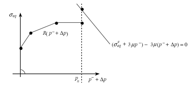
The implicit discretization of the behavioral relationship leads to solving an equation in \(\Delta p\) (see § 3.3):
\({\sigma }_{\mathrm{eq}}^{e}-3\mu \Delta p -R({p}^{-}+\Delta p )=0\)
The equation is solved exactly by taking advantage of piecewise linearity.
We first examine whether the solution could be outside the limits of the discretization points of the curve \(R(p)\), that is to say, if \(p\ge {p}_{n}\) is a possible solution. For this:
If \({\sigma }_{\mathrm{eq}}^{e}+3\mu ({p}^{-}-{p}_{n})-{\sigma }_{n}\ge 0\), then we are in the following situation:
if the extension to the right is linear then: \(\Delta p=\frac{{\sigma }_{\text{eq}}^{e}-{H}_{n-1}}{{\alpha }_{n-1}+3\mu }\)
with: \({\alpha }_{n-1}=\frac{{\sigma }_{n}-{\sigma }_{n-1}}{{p}_{n}-{p}_{n-1}}\text{}{H}_{n-1}={\sigma }_{n-1}+{\alpha }_{n-1}\left({p}^{-}-{p}_{n-1}\right)\)
if the extension is constant: \(\Delta p=\frac{{\sigma }_{\mathit{eq}}^{e}-{\sigma }_{n}}{3\mu }\)
otherwise, the solution \(p\) is to be found in the \([{p}_{i},{p}_{i+1}]\) interval such as:
\({\sigma }_{i+1}>{\sigma }_{\text{eq}}^{e}+3\mu \left({p}^{-}-{p}_{i+1}\right)\) and \({\sigma }_{i}\le {\sigma }_{\text{eq}}^{e}+3\mu \left({p}^{-}-{p}_{i}\right)\)
so the solution is: \(\Delta p=\frac{{\sigma }_{\text{eq}}^{e}-{H}_{i}}{{\alpha }_{i}+3\mu }\text{et}{p}^{-}+\Delta p\in \left[{p}_{i},{p}_{i+1}\right]\)
with:
\({\alpha }_{i}=\frac{{\sigma }_{i+1}-{\sigma }_{i}}{{p}_{i+1}-{p}_{i}}\text{;}{H}_{i}={\sigma }_{i}+{\alpha }_{i}\left({p}^{-}-{p}_{i}\right)\text{pour}i=1\text{à}n-1\)
Isotropic work hardening under plane stress
In this case, the system to be solved includes one more equation: \(\Delta {\sigma }_{33}=0\) .We then obtain the following system:
\(\{\begin{array}{c}2\mu \Delta \tilde{\varepsilon }-\Delta \tilde{\sigma }=\frac{3}{2}2\mu \Delta p\frac{{\tilde{\sigma }}^{-}+\Delta \tilde{\sigma }}{{({\sigma }^{-}+\Delta \sigma )}_{\text{eq}}}\\ \text{tr}\Delta \sigma =3K\text{tr}\Delta \varepsilon \\ {({\sigma }^{-}+\Delta \sigma )}_{\text{eq}}-R({p}^{-}+\Delta p)\le 0\\ \Delta p=0\text{si}{({\sigma }^{-}+\Delta \sigma )}_{\text{eq}}<R({p}^{-}+\Delta p)\\ \begin{array}{}\Delta p\ge 0\text{si}{({\sigma }^{-}+\Delta \sigma )}_{\text{eq}}=R({p}^{-}+\Delta p)\\ \Delta {\sigma }_{\text{33}}=0\end{array}\end{array}\)
With this assumption, \(\Delta \varepsilon\) is not fully known: \(\Delta {\varepsilon }_{33}\) cannot be calculated only from \(\Delta {u}_{i}^{n}\).
Note:
In the case of models other than C_PLAN, so for example for shell models (DKT, * COQUE_3D), the hypotheses on transverse shear terms \(\Delta {\sigma }_{13}\) and \(\Delta {\sigma }_{23}\) are defined by these models (in general, the behavior associated with transverse shear is linear, elastic and decoupled from the equations above). Therefore, these terms are not taken into account here.
We pose \(\Delta \varepsilon =\Delta {\varepsilon }^{q}+\Delta {\varepsilon }^{y}\) with \(\Delta {\varepsilon }^{q}\) fully known from \(\Delta {u}_{i}^{n}\) and elasticity, so \(\Delta {\varepsilon }_{\text{33}}^{q}=-\frac{\nu }{1-\nu }(\Delta {\varepsilon }_{\text{11}}^{q}+\Delta {\varepsilon }_{\text{22}}^{q})\text{et}\Delta {\varepsilon }^{y}=(\begin{array}{ccc}0& 0& 0\\ 0& 0& 0\\ 0& 0& \Delta y\end{array})\) is unknown.
Compared to the previous system, there is an additional unknown, \(\Delta y\).
If \({({\tilde{\sigma }}^{-}+\Delta \tilde{\sigma })}_{\text{eq}}<R({p}^{-}+\Delta p)\text{alors}\Delta p=0\) so \(2\mu \Delta \tilde{\varepsilon }=\Delta \tilde{\sigma },\) that is to say \(\Delta y =0\text{.}\)
Otherwise, the resolution technique is to express \(\Delta y\) in terms of \(\Delta p\). We then get a non-linear scalar equation in \(\Delta p\).
We ask: “\({\tilde{\sigma }}^{e}=\frac{2\mu }{2{\mu }^{-}}{\tilde{\sigma }}^{-}+2\mu \Delta {\tilde{\varepsilon }}^{q}\). In the same way as for integration without plane constraints, we obtain:
\({\tilde{\sigma }}_{e}+2\mu {\stackrel{}{\Delta \tilde{\varepsilon }}}^{y}=({\tilde{\sigma }}^{-}+\stackrel{}{\Delta \tilde{\sigma }})(1+\frac{3\mu \Delta p}{R(p+\Delta p)})\).
But this expression involves an additional unknown \(\Delta y\): In particular:
\({\tilde{\sigma }}_{33}+2\mu \Delta {\tilde{\varepsilon }}_{33}^{y}=({\tilde{\sigma }}_{33}^{-}+\Delta {\tilde{\sigma }}_{33})(1+\frac{3\mu \Delta p}{R(p+\Delta p)})\)
gold
\(\Delta {\tilde{\varepsilon }}_{33}^{y}=\frac{2}{3}\Delta y\)
and \(\mathrm{tr}({\sigma }^{-}+\Delta \sigma )=3K\mathrm{tr}{\Delta \varepsilon }^{q}+3{K}^{+}\Delta y+\frac{3{K}^{+}}{3{K}^{-}}\mathrm{tr}{\sigma }^{-}-3{K}^{+}\Delta {\varepsilon }^{\mathrm{th}}\)
Like:
\({\tilde{\sigma }}_{\text{33}}^{e}+\Delta {\tilde{\sigma }}_{33}={\sigma }_{\text{33}}^{e}+\Delta {\sigma }_{33}=\frac{\mathrm{tr}({\sigma }^{-}+\Delta \sigma )}{3}=0-\frac{\mathrm{tr}({\sigma }^{-}+\Delta \sigma )}{3}\)
An equation linking \(\Delta y\) and \(\Delta p\) is obtained:
\({\tilde{\sigma }}_{33}+2\frac{2}{3}\Delta y=(1+\frac{3\mu \Delta p}{R(p+\Delta p)})(\frac{-\mathrm{tr}{\sigma }_{e}-3K\Delta y}{3})\)
with:
\(\mathrm{tr}{\sigma }_{e}=\frac{3K}{3{K}^{-}}\mathrm{tr}{\sigma }^{-}+3K\mathrm{tr}\Delta {\varepsilon }^{q}-3K\Delta {\varepsilon }^{\mathrm{th}}\)
That is:
\(\Delta y(\frac{4\mu }{3}+K(1+\frac{3\mu \Delta p}{R({p}^{-}+\Delta p)}))={\tilde{\sigma }}_{\text{33}}^{e}-\frac{\text{tr}{\sigma }_{e}}{3}(1+\frac{3\mu \Delta p}{R({p}^{-}+\Delta p)})\)
noticing that:
\({\tilde{\sigma }}_{\text{33}}^{e}={\sigma }_{\text{33}}^{e}-\frac{\text{tr}{\sigma }_{e}}{3}=0-\frac{\text{tr}{\sigma }_{e}}{3}\)
and by explaining \(\mu ,K\), we get:
\(\Delta y =\frac{3(1-2\nu )\Delta p }{E\Delta p +2(1-\nu )R(p+\Delta p )}{\tilde{\sigma }}_{\text{33}}^{e}\)
to be added to the equation in \(\Delta p\) (identical to the previous cases):
\({(\tilde{{\sigma }^{e}}+2\mu {\Delta \tilde{\varepsilon }}^{y})}_{\mathrm{eq}}-3\mu \Delta p-R({p}^{-}+\Delta p)=0\)
where \(\Delta y\) is expressed in terms of \(\Delta p\) since: \({\stackrel{}{\Delta \tilde{\varepsilon }}}^{y}=\frac{\Delta y }{3}(\begin{array}{ccc}-1& & \\ & -1& \\ & & 2\end{array})\)
The scalar equation in \(\Delta p\) obtained in this way is still non-linear. This equation is solved by a method for finding function zeros, based on a secant algorithm. Once the solution \(\Delta p\) is known, \(\Delta y\) is calculated and then \(\sigma\) is calculated.