4. Von Mises relationship to linear kinematic work hardening#
4.1. Expression of the behavioral relationship, general case#
This relationship is obtained by the keyword VMIS_CINE_LINE from the keyword factor COMPORTEMENT.
It is written (always in small deformations):
\(\{\begin{array}{c}{\dot{\varepsilon }}^{p}=\frac{3}{2}\dot{p}\frac{\tilde{\sigma }-\tilde{X}}{{(\sigma -X)}_{\text{eq}}}=\frac{3}{2}\dot{p}\frac{\tilde{\sigma }-X}{{(\sigma -X)}_{\text{eq}}}=\dot{\varepsilon }-\stackrel{·}{\stackrel{}{{A}^{-1}\sigma }}-{\dot{\varepsilon }}^{\text{th}}\\ X=C{\varepsilon }^{p},{\varepsilon }^{\text{th}}=\alpha (T-{T}_{\text{ref}})\mathrm{Id}\\ {(\sigma -X)}_{\text{eq}}-{\sigma }_{y}\le 0\\ \{\begin{array}{c}\dot{p}=0\text{si}{(\sigma -X)}_{\text{eq}}-{\sigma }_{y}\le 0\\ \dot{p}\ge 0\text{si}{(s-X)}_{\text{eq}}-{\sigma }_{y}=0\end{array}\end{array}\) eq 4.1-1
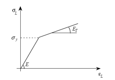
\({\sigma }_{y}\) is the elastic limit (the choice of \({\sigma }_{y}\) is up to the user: it can correspond to the end of the linearity of the real tension curve, or to a regulatory or conventional elastic limit… Anyway, here we use the only value defined under ECRO_LINE).
\(C\) is the work-hardening coefficient deduced from the data by a simple tensile test.
In this case (uniaxial stress tensor, isochoric and orthotropic plastic deformation tensor):
\(\sigma =(\begin{array}{ccc}{\sigma }_{L}& 0& 0\\ 0& 0& 0\\ 0& 0& 0\end{array})\) \(X=(\begin{array}{ccc}{X}_{L}& 0& 0\\ 0& -\frac{{X}_{L}}{2}& 0\\ 0& 0& -\frac{{X}_{L}}{2}\end{array})\)
\({(\sigma -X)}_{\mathrm{eq}}={\sigma }_{L}-\frac{3}{2}{X}_{L}\) and \({X}_{L}=C{\varepsilon }_{L}^{p}=C({\varepsilon }_{L}-\frac{{\sigma }_{L}}{E})\)
The material data is that provided under the keyword factor ECRO_LINE or ECRO_LINE_FO of the operator DEFI_MATERIAU:
/ECRO_LINE =_F (D_SIGM_EPSI = \({E}_{T}\), SY = \({\sigma }_{y}\))
/ECRO_LINE_FO =_F (D_SIGM_EPSI = \({E}_{T}\), SY = \({\sigma }_{y}\))
ECRO_LINE_FO corresponds to the case where \({E}_{T}\) and \({\sigma }_{y}\) depend on the temperature and are then calculated for the temperature of the current Gauss point.
Young’s modulus \(E\) and Poisson’s ratio are those provided under the keywords ELAS or ELAS_FO factors.
For \({\varepsilon }_{L}>\frac{{\sigma }_{y}}{E}\) \({\sigma }_{L}={\sigma }_{y}+{E}_{T}({\varepsilon }_{L}-\frac{{\sigma }_{y}}{E})\),
but we also have:
\(\{\begin{array}{c}{\sigma }_{L}-\frac{3}{2}{X}_{L}={\sigma }_{y}\\ {X}_{L}=C({\varepsilon }_{L}-\frac{{\sigma }_{L}}{E})\end{array}\)
Hence, by eliminating \({X}_{L}\) and identifying:
\(C=\frac{2}{3}\frac{E{E}_{T}}{E-{E}_{T}}\).
4.2. Expression of the behavioral relationship in 1D#
For performance reasons, the relationship is also written in 1D for use with finite elements such as multi-fiber beams. The preceding equations are identical, the quantities \({\sigma }_{L}\), \({X}_{L}\), and \({\varepsilon }_{L}\) are scalars.
The material data is that provided under the keyword factor ECRO_LINE of the DEFI_MATERIAU operator [U4.43.01]:
/ECRO_LINE =_F (
♦ D_SIGM_EPSI = \({E}_{T}\) [Real]
♦ SY = \({\sigma }_{y}\) [Real]
◊ SIGM_ELS = symbols [Real]
◊ EPSI_ELU =epsielu [Real]
The sigm_els and espi_elu operands make it possible to define the limits that correspond to the service limit and ultimate states, classically used during studies in civil engineering.
◊ SIGM_ELS =sgels
Definition of the service limit constraint.
◊ EPSI_ELU =epelu
Definition of ultimate limit deformation.
These terminals are mandatory when using the Ecro_Cine_1D behavior (Cf. [:ref:` U4 . 5 1. 11 < U4 . 5 1. 11 >`] Non-linear behaviors, [U4.42.07] DEFI_MATER_GC). In the other cases they are not taken into account.
The supported modeling is 1D, the number of internal variables is 6.
\(\mathrm{V1}\): Criterion ELS: CRITELS. This variable gives information about the service limit state. This variable represents the absolute value of the stress divided by the limiting stress at ELS of the material. If this variable is in \(\mathrm{[}\mathrm{0,}1\mathrm{]}\) the material respects ELS.
\(\mathrm{V2}\): Criterion ELU: CRITELU. This variable gives information about the ultimate limit state. This variable represents the absolute value of the total deformation divided by the limiting deformation at ELU of the material. If this variable is in \(\mathrm{[}\mathrm{0,}1\mathrm{]}\) the material respects ELU.
\(\mathrm{V3}\): Kinematic work hardening: XCINXX. In 1D only a scalar is required.
\(\mathrm{V4}\): Plastic indicator: INDIPLAS. Indicates whether the material has exceeded the elastic criterion.
\(\mathit{V5}\): non-recoverable dissipation: DISSIP. During seismic calculations it may be useful for the user to know the energy dissipated that cannot be recovered. The variable dissip represents the accumulation of non-recoverable energy. The non-recoverable energy increment is written in the form:
\(\Delta \mathit{Eg}\mathrm{=}\frac{1}{2}({E}^{\text{+}}\Delta \varepsilon –({\sigma }^{\text{+}}\mathrm{-}{\sigma }^{\text{-}}))\Delta \varepsilon\)
\(\mathit{V6}\): thermodynamic dissipation: DISSTHER. The thermodynamic dissipation increment is written in the form: \(\Delta \mathit{Eg}\mathrm{=}{\sigma }_{y}\dot{p}\).
4.3. Tangent operator. Option RIGI_MECA_TANG#
The aim of this paragraph is to calculate the tangent operator \({K}_{i-1}\) (calculation option RIGI_MECA_TANG called at the first iteration of a new load increment) from the results known at the previous moment \({t}_{i-1}\).
To do this, if the stress tensor at \({t}_{i-1}\) is on the border of the elasticity domain, we write the condition:
\(\dot{f}=0\)
which should be checked (for the ongoing problem in time) in conjunction with the condition:
\(f=0\)
with
\(f=f({\sigma }^{-},{X}^{-})={({\sigma }^{-}-{X}^{-})}_{\text{eq}}-{\sigma }_{y}\)
If, on the other hand, the stress tensor at \({t}_{i-1}\) is within the domain, \(f<0\), then the tangent operator is the elasticity operator.
We ask:
\({\sigma }^{\text{dev}}={\tilde{\sigma }}^{-}-{X}^{-}\text{et}\gamma =\{\begin{array}{c}1\text{si}{({\sigma }^{-}-{X}^{-})}_{\text{eq}}-{\sigma }_{y}=0(\text{variable interne}\chi )\\ 0\text{sinon}\end{array}\)
The speed problem is written in this case:
\(\{\begin{array}{c}{\dot{\varepsilon }}^{p}=\{\begin{array}{c}\frac{1}{2\mu }\frac{3}{2}{(\frac{2\mu }{{\sigma }_{y}})}^{2}\frac{((\tilde{\sigma }-X)\text{.}\dot{\tilde{\varepsilon }})(\tilde{\sigma }-X)}{C+2\mu }\text{si}(\sigma -X)-{\sigma }_{y}=0\\ 0\text{si}{(s-X)}_{\mathrm{eq}}-{\sigma }_{y}<0\end{array}\\ {\dot{\sigma }}_{\text{ij}}=K{\dot{\varepsilon }}_{\text{kk}}{\delta }_{\text{ij}}+2\mu ({\dot{\tilde{\varepsilon }}}_{\text{ij}}-{\dot{\varepsilon }}_{\text{ij}}^{p})\end{array}\)
The tangent operator links the virtual deformation vector \({\varepsilon }^{\ast }\) to a virtual stress vector \({\sigma }^{\ast }\).
The tangent stiffness matrix is written for elastic behavior:
\({\sigma }^{\ast }=(K\overrightarrow{1}\otimes \overrightarrow{1}+2\mup ){\varepsilon }^{\ast }\)
and for plastic behavior:
\({\sigma }^{\ast }=(K\overrightarrow{1}\otimes \overrightarrow{1}+2\mup -{C}_{p}s\otimes s){\varepsilon }^{\ast }\)
with \(s\) the vector of deviatory constraints associated with \({\sigma }^{\mathrm{dev}}\) defined by:
\({s}^{T}=({\sigma }_{\text{11}}^{\mathrm{dev}},{\sigma }_{\text{22}}^{\mathrm{dev}},{\sigma }_{\text{33}}^{\mathrm{dev}},\sqrt{2}{\sigma }_{\text{12}}^{\mathrm{dev}},\sqrt{2}{\sigma }_{\text{23}}^{\mathrm{dev}},\sqrt{2}{\sigma }_{\text{31}}^{\mathrm{dev}})\)
and:
\({C}_{p}=\gamma \frac{3}{2}{(\frac{2\mu }{{\sigma }_{y}})}^{2}\frac{1}{2\mu +C}\)
In the case of the first loading increment, therefore if the state at the previous instant corresponds to an initial unconstrained state, the tangent operator is identical to the elasticity operator.
4.4. Calculation of constraints and internal variables#
The direct implicit discretization of continuous relationships leads to the resolution of:
\(\{\begin{array}{c}2\mu \Delta {\varepsilon }^{p}=2\mu (\Delta \tilde{\varepsilon }+\frac{{\tilde{\sigma }}^{-}}{2{\mu }^{-}}-\frac{\tilde{\sigma }}{2\mu })=\frac{3}{2}2\mu \Delta p\frac{\tilde{\sigma }-X}{{\sigma }_{y}}\\ X=\frac{C}{{C}^{-}}{X}^{-}+C\Delta {\varepsilon }^{p}\\ {(\sigma -X)}_{\text{eq}}\le {\sigma }_{y}\\ \Delta p=0\text{si}{(\sigma -X)}_{\text{eq}}<{\sigma }_{y}\\ \Delta p\ge 0\text{sinon}\\ \text{tr}({\sigma }^{-}+\Delta \sigma )=\frac{3K}{3{K}^{-}}\text{tr}{\sigma }^{-}+3K\text{tr}\Delta \varepsilon -3K\text{tr}\Delta {\varepsilon }^{\text{th}}\end{array}\)
We are still asking:
\({\tilde{\sigma }}^{e}=\frac{2\mu }{2{\mu }^{-}}{\tilde{\sigma }}^{-}+2\mu \Delta \tilde{\varepsilon }-\frac{C}{{C}^{-}}{X}^{-}\).
The first equation is also written as:
\((2\mu \Delta \tilde{\varepsilon }+\frac{2\mu }{2{\mu }^{-}}{\tilde{\sigma }}^{-})=\tilde{\sigma }+\frac{3}{2}2\mu \Delta p \frac{\tilde{\sigma }-X}{{\sigma }_{y}}\)
subtracting \(X=\frac{C}{{C}^{-}}{X}^{-}+C\Delta {\varepsilon }^{p}\) from each term, we get:
\(2\mu \Delta \tilde{\varepsilon }+\frac{2\mu }{2{\mu }^{-}}{\tilde{\sigma }}^{-}-\frac{C}{{C}^{-}}{X}^{-}=\tilde{\sigma }-X+\frac{3}{2}2\mu \Delta p \frac{\tilde{\sigma }-X}{{\sigma }_{y}}+C\Delta {\varepsilon }^{P}\)
or again, using the flow law:
\({\tilde{\sigma }}^{e}=(\tilde{\sigma }-X)(\text{1+}\frac{3}{2}(2\mu +C)\frac{\Delta p }{{\sigma }_{y}})\)
We get another scalar equation in \(\Delta p\) by taking the equivalent Von Mises values:
\({\sigma }_{\text{eq}}^{e}={\sigma }_{y}+\frac{3}{2}(2\mu +C)\Delta p\)
which directly gives:
\(\Delta p =\frac{{\sigma }_{\text{eq}}^{e}-{\sigma }_{y}}{\frac{3}{2}(2\mu +C)}\)
And \(\sigma\) is obtained by: \(\tilde{\sigma }=\frac{2\mu }{2{\mu }^{-}}{\tilde{\sigma }}^{-}+2\mu \Delta \tilde{\varepsilon }+2\mu \Delta {\varepsilon }^{p}\)
Noticing that: \(\stackrel{}{\Delta {\varepsilon }^{p}}=\frac{3}{2}\stackrel{}{\Delta p }\frac{\tilde{\sigma }-X}{{\sigma }_{y}}=\frac{3}{2}\stackrel{}{\Delta p }\frac{{\tilde{\sigma }}^{e}}{{\sigma }_{\text{eq}}^{e}}\) because: \(\frac{\tilde{\sigma }-X}{{\sigma }_{y}}=\frac{{\tilde{\sigma }}^{e}}{{\sigma }_{\text{eq}}^{e}}\)
So we have:
\(\tilde{\sigma }=\frac{2\mu }{2{\mu }^{-}}{\tilde{\sigma }}^{-}+2\mu \stackrel{}{\Delta \tilde{\varepsilon }}-\frac{2\mu }{2\mu +C}\frac{{({s}_{\text{eq}}^{e}-{\sigma }_{y})}_{\text{+}}}{{\sigma }_{\text{eq}}^{e}}\text{.}{\tilde{\sigma }}^{e}\)
The \(X\) internal variables are calculated by:
\(X=\frac{C}{{C}^{-}}{X}^{-}+C\Delta {\varepsilon }^{p}=\frac{C}{{C}^{-}}{X}^{-}+\frac{3}{2}C\Delta p\frac{{\tilde{\sigma }}^{e}}{{\sigma }_{\text{eq}}^{e}}\)
**Note:***Special case of plane stresses. *
The direct consideration of the hypothesis of plane stresses in the integration of the Von Mises model with linear kinematic work hardening has not been done in Code_Aster. To take into account this hypothesis, that is to say to use Von Mises elastoplastic behavior with linear kinematic work hardening (Prager’s law) with the models C_PLAN, DKT, COQUE_3D, COQUE_AXIS,, COQUE_D_PLAN,,,,, COQUE_C_PLAN,,, TUYAU, TUYAU_6M, we can:
or use the static condensation method (due to R. de Borst [R5.03.03]) which makes it possible to obtain a plane state of constraints at the convergence of the global iterations of the Newton algorithm;
or use the VMIS_ECMI_LINE behavior (cf. [R5.03.16]).
4.5. Tangent operator. Option FULL_MECA#
Option FULL_MECA allows you to calculate the tangent matrix \({K}_{i}^{n}\) at each iteration. The tangent operator that is used to construct it is calculated directly on the previous discretized system (we note for simplicity: \(\tilde{\sigma }=\tilde{{\sigma }^{-}}+\Delta \tilde{\sigma },p={p}^{-}+\Delta p\)) and we write the expressions only in the isothermal case.
We ask \({\sigma }^{\mathrm{dev}}=\tilde{\sigma }-X\) and \(\gamma =\{\begin{array}{c}1\text{si}\Delta p>0\text{et}(\tilde{\sigma }-X)\text{.}\Delta \tilde{\varepsilon }\ge 0\\ 0\text{sinon}\end{array}\)
The tangent operator links the virtual deformation vector \({\mathrm{\epsilon }}^{\ast }\) to the virtual stress vector \({\mathrm{\sigma }}^{\ast }\). So the tangent stiffness matrix is written as:
\({\mathrm{\sigma }}^{\ast }=\left(K\vec{1}\otimes \vec{1}+2\mu {a}_{2}P-{C}_{p}\mathrm{s}\otimes \mathrm{s}\right){\mathrm{\epsilon }}^{\ast }\)
with \(s\) the constraint vector associated with \({\sigma }^{\mathrm{dev}}\) by:
\({s}^{T}=({\sigma }_{\text{11}}^{\mathrm{dev}},{\sigma }_{\text{22}}^{\mathrm{dev}},{\sigma }_{\text{33}}^{\mathrm{dev}},\sqrt{2}{\sigma }_{\text{12}}^{\mathrm{dev}},\sqrt{2}{\sigma }_{\text{23}}^{\mathrm{dev}},\sqrt{2}{\sigma }_{\text{31}}^{\mathrm{dev}})\)
and:
\({C}_{p}=\gamma \frac{3}{2}{(\frac{2\mu }{{\sigma }_{y}})}^{2}\frac{1}{2\mu +C}{a}_{1}\) with \({a}_{1}=\frac{1}{1+\frac{3}{2}\frac{(2\mu +C)\mathrm{\Delta }p}{{\sigma }_{y}}}\) and \({a}_{2}={a}_{1}(1+\frac{3}{2}C\frac{\Delta p }{{\sigma }_{y}})\)
4.6. Model VMIS_CINE_LINE Internal Variables#
There are 7 internal variables:
the :math:`` tensor stored on 6 components,
the scalar variable \(\khi\).