3. Von Mises relationship to isotropic work hardening#

3.1. Expression of behavioral relationships#

These relationships are obtained by the keywords VMIS_ISOT_LINE, VMIS_ISOT_TRAC, and VMIS_ISOT_PUIS.

These relationships are described here in small deformations (DEFORMATION =” PETIT “):

\(\begin{array}{c}\{\begin{array}{c}{\dot{\mathrm{\epsilon }}}^{p}=\frac{3}{2}\dot{p}\mathrm{.}\frac{\stackrel{~}{\mathrm{\sigma }}}{{\mathrm{\sigma }}_{\text{eq}}}=\dot{\mathrm{\epsilon }}-\stackrel{·}{\stackrel{⏞}{{A}^{-1}\mathrm{\sigma }}}-{\dot{\mathrm{\epsilon }}}^{\text{th}}\\ {\mathrm{\sigma }}_{\text{eq}}-R\left(p\right)\le 0\\ (\begin{array}{c}\dot{p}=0\text{si}{\mathrm{\sigma }}_{\text{eq}}-R\left(p\right)<0\\ \dot{p}\ge 0\text{si}{\mathrm{\sigma }}_{\text{eq}}-R\left(p\right)=0\end{array}\end{array}\\ \begin{array}{cc}{\dot{\mathrm{\epsilon }}}^{p}\mathrm{:}& \text{vitesse de déformation plastique,}\\ p\mathrm{:}& \text{déformation plastique cumulée}\mathrm{:}p=\sqrt{\frac{2}{3}{\dot{\mathrm{\epsilon }}}^{p}\mathrm{:}{\dot{\mathrm{\epsilon }}}^{p}}\\ {\mathrm{\epsilon }}^{\text{th}}\mathrm{:}& \text{déformation d'origine thermique}\mathrm{:}{\mathrm{\epsilon }}^{\text{th}}=\mathrm{\alpha }\left(T-{T}_{\text{ref}}\right)\text{Id}\end{array}\end{array}\)

The work hardening function \(R(p)\) is deduced from a simple monotonic and isothermal tensile test.

For the von Mises relation to work hardening, the equivalent plastic deformation \({\mathrm{\epsilon }}_{\mathit{eq}}^{p}=\sqrt{\frac{3}{2}{\stackrel{~}{\mathrm{\epsilon }}}_{ij}^{p}{\stackrel{~}{\mathrm{\epsilon }}}_{ij}^{p}}\), the cumulative plastic deformation \(p\) and the work hardening variable \(R(p)\), coincide. code_aster saves the same value of these three terms in the internal variable « EPSPEQ » (equivalent plastic deformation).

The user can choose linear work hardening (relationship VMIS_ISOT_LINE) or a traction curve given either point by point (relationship VMIS_ISOT_TRAC), or by an analytical expression (relationship) or by an analytical expression (relationship) or a traction curve given by point (relationship).

VMIS_ISOT_PUIS).

Behavioral law VMIS_JOHN_COOK differs from the previous ones in the sense that the work hardening function depends on the rate of cumulative plastic deformation and on the temperature.

These relationships are described here in small deformations (DEFORMATION =” PETIT “):

\(\begin{array}{c}\{\begin{array}{c}{\dot{\mathrm{\epsilon }}}^{p}=\frac{3}{2}\dot{p}\frac{\stackrel{~}{\mathrm{\sigma }}}{{\sigma }_{\text{eq}}}=\dot{\mathrm{\epsilon }}-\stackrel{·}{\stackrel{⏞}{{A}^{-1}\mathrm{\sigma }}}-{\dot{\mathrm{\epsilon }}}^{\text{th}}\\ {\sigma }_{\text{eq}}-R\left(p,\dot{p},T\right)\le 0\\ \{\begin{array}{c}\dot{p}=0\text{si}{\sigma }_{\text{eq}}-R\left(p,\dot{p},T\right)<0\\ \dot{p}\ge 0\text{si}{\sigma }_{\text{eq}}-R\left(p,\dot{p},T\right)=0\end{array}\end{array}\\ \begin{array}{cc}{\dot{\mathrm{\epsilon }}}^{p}\mathrm{:}& \text{vitesse de déformation plastique,}\\ p\mathrm{:}& \text{déformation plastique cumulée,}\\ \dot{p}\mathrm{:}& \text{vitesse de déformation plastique cumulée,}\\ {\mathrm{\epsilon }}^{\text{th}}\mathrm{:}& \text{déformation d'origine thermique}\mathrm{:}{\mathrm{\epsilon }}^{\text{th}}=\alpha \left(T-{T}_{\text{ref}}\right)\text{Id}\end{array}\end{array}\)

The work hardening function \(R(p,\dot{p},T)\) is derived from a series of simple monotonic tensile tests at different deformation rates and at different temperatures.

3.1.1. Relationship VMIS_ISOT_LINE#

Material characteristic data are those provided under the keyword factor ECRO_LINE or ECRO_LINE_FO of the DEFI_MATERIAU [U4.43.01] operator.

/ECRO_LINE =_F (D_SIGM_EPSI = \({E}_{T}\), SY = \({\sigma }_{y}\))

/ECRO_LINE_FO =_F (D_SIGM_EPSI = \({E}_{T}\), SY = \({\sigma }_{y}\))

ECRO_LINE_FO corresponds to the case where \({E}_{T}\) and \({\sigma }_{y}\) depend on the temperature and are then calculated for the temperature of the current Gauss point.

Young’s modulus \(E\) and Poisson’s ratio \(\nu\) are those provided under the keywords factors ELAS or ELAS_FO.

In this case the traction curve is as follows:

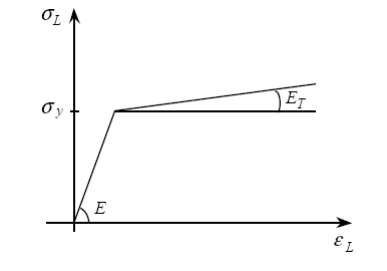
That is to say:

\((\begin{array}{c}{\sigma }_{L}=E{\varepsilon }_{L}\text{si}{\varepsilon }_{L}\le \frac{{\sigma }_{y}}{E}\\ {\sigma }_{L}={\sigma }_{y}+{E}_{T}({\varepsilon }_{L}-\frac{{\sigma }_{y}}{E})\text{si}{\varepsilon }_{L}\ge \frac{{\sigma }_{y}}{E}\end{array}\)

Note:

\({\sigma }_{y}\) is the elastic limit (the choice of \({\sigma }_{y}\) is up to the user: it can correspond to the end of the linearity of the real tension curve, or to a regulatory or conventional elastic limit. Anyway, here we use the only value defined under ECRO_LINE) .

When the criterion is reached we have: \({\sigma }_{\mathrm{eq}}-R(p)=0\). To identify \(R(p)\), we use the properties of the uniaxial stress state:

\(\sigma =(\begin{array}{ccc}{\sigma }_{L}& 0& 0\\ 0& 0& 0\\ 0& 0& 0\end{array})\). so \(\begin{array}{c}{\sigma }_{\text{eq}}={\sigma }_{L}\\ p={\varepsilon }_{L}^{P}={\varepsilon }_{L}-\frac{{\sigma }_{L}}{E}\end{array}\) and the criterion is written as: \({\sigma }_{L}-R(p)=0\)

\({\sigma }_{L}-{\sigma }_{y}={E}_{T}({\varepsilon }_{L}-\frac{{\sigma }_{y}}{E})={E}_{T}(\frac{{\sigma }_{L}}{E}+p-\frac{{\sigma }_{y}}{E})\)

therefore

\(({\sigma }_{L}-{\sigma }_{y})(1-\frac{{E}_{T}}{E})={E}_{T}p\) or \(({\sigma }_{L}-{\sigma }_{y})=\frac{{E}_{T}\mathrm{.}E}{(E-{E}_{T})}p\)

Hence the linear work hardening function: \(R(p)=\frac{{E}_{T}E}{E-{E}_{T}}p+{\sigma }_{y}\)

3.1.2. Relationship VMIS_ISOT_TRAC#

The material data is that provided under the keyword factor TRACTION =_F (SIGM = f), from the operator DEFI_MATERIAU.

f is a function with one or two variables representing simple traction curves. The first variable is necessarily deformation, the second, if it exists, is temperature (parameter of a sheet). For each temperature, the traction curve must be such that:

the abscissa (true deformations) are strictly increasing,
the first point on the curve corresponds to \(({ϵ}_{\mathrm{1,}}{\sigma }_{y})\) where \({ϵ}_{1}\ne 0\) and \({\sigma }_{y}\) is the elastic limit,
the slope between 2 successive points is less than the elastic slope between 0 and the first point of the curve \((E={\sigma }_{y}/{ϵ}_{1})\).

To interpolate with respect to temperature, Code_Aster first transforms all \(\sigma =f(ϵ)\) curves given by the user into \(\sigma (p)=R(p)\) curves in the following way: if \(E\) is the elastic slope between 0 and the first point of the curve \(({ϵ}_{\mathrm{1,}}{\sigma }_{y})\) (where \({ϵ}_{1}\ne 0\) and \({\sigma }_{y}\) is the elastic limit), any point on the curve \(({ϵ}_{i},{\sigma }_{i})\) becomes the point \(({p}_{i},{\sigma }_{i})\) with \({p}_{i}={ϵ}_{i}-{\sigma }_{i}/E\) (from where \({p}_{1}=0\)). Let \(\theta\) be the temperature in question, if there is \(k\) such as \(\theta \in [:ref:`{\theta }_{k},{\theta }_{k+1} <{\theta }_{k},{\theta }_{k+1}>\)] where :math:`k designates the index of the traction curves contained in the water table, we build point by point the curve \(R(p,\theta )\) by interpolating from \(R(p,{\theta }_{k})\) and \(R(p,{\theta }_{k+1})\) for all the values of \(p\) for all the values of of the meeting of the values of the abscissa of curves \(k\) and \(k+1\) (in the case where these two curves are extended linearly or by a constant function):

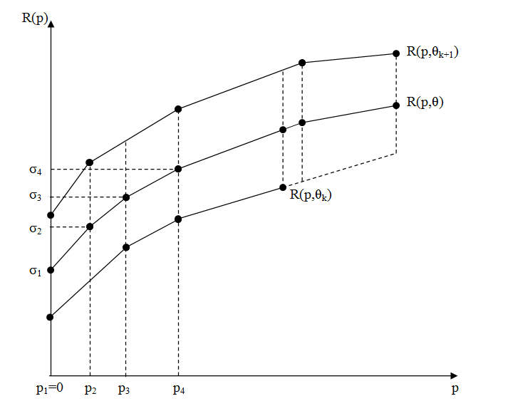
If \({n}_{k}\) and \({n}_{k+1}\) are the numbers of points of the curves \(k\) and \(k+1\), the number of points \(n\) of the curve \(R(p,\theta )\) is equal in the general case to \({n}_{k}+{n}_{k+1}-1\) (case where all the non-zero abscissas are distinct).

If \(\theta\) is outside the definition intervals of the traction curves, one extrapolates in accordance with the extensions specified by the user in DEFI_NAPPE [U4.21.03] and according to the previous principle.

Note:

To avoid generating significant approximation errors or even obtaining bad traction curves by extrapolation, it is best not to use linear extensions in DEFI_NAPPE.

In the case where the extension of the shortest curve is « EXCLU », the interpolation is stopped at this point and the extension of the interpolated curve is also « EXCLU ».

In all cases, a piecewise linear work hardening function is therefore obtained:

\(R(p,q)={s}_{i}+\frac{{s}_{i+1}-{s}_{i}}{{p}_{i+1}-{p}_{i}}(p-{p}_{i})\) for \(p\in [:ref:`{p}_{i},{p}_{i+1} <{p}_{i},{p}_{i+1}>\)] for :math:`i+1le n, with \({p}_{1}=0\)

The Young’s modulus corresponding to temperature \(\theta\) is calculated as follows:

\(E={E}_{k}+\frac{q-{q}_{k}}{{q}_{k+1}-{q}_{k}}({E}_{k+1}-{E}_{k})\)

where, for \(i=k\) or \(i=k+1\), \({E}_{i}\) is the elastic slope between \(0\) and the first point on the \(\sigma =f(\epsilon )\) curve corresponding to the temperature \({\theta }_{i}\).

It is this Young’s module that is used in the integration of the behavioral relationship.

The elastic limit at temperature \(\theta\) is equal to:

\({\sigma }_{y}=R(\mathrm{0,}\theta )={\sigma }_{1}\)

The user must also give the Poisson’s ratio \(\nu\) and a fictional Young’s modulus (which is only used to calculate the elastic stiffness matrix if the keyword NEWTON =_F (MATRICE =” ELASTIQUE “) is present in STAT_NON_LINE) by the keywords:

/ELAS =_F (NU = \(\nu\), E = \(E\))

/ELAS_FO =_F (NU = \(\nu\), E = \(E\))

3.1.3. Relationship VMIS_ISOT_PUIS#

The material data is that provided under the keyword factor ECRO_PUIS or ECRO_PUIS_FO of the operator DEFI_MATERIAU [U4.43.01].

ECRO_PUIS =_F (SY= \({\sigma }_{y}\), A_PUIS =a, N_PUIS =n)

The work hardening curve is deduced from the uniaxial curve relating the deformations to the stresses, whose expression is:

\(\mathrm{\epsilon }=\frac{\mathrm{\sigma }}{E}+a\frac{{\mathrm{\sigma }}_{y}}{E}{\left(\frac{\mathrm{\sigma }-{\mathrm{\sigma }}_{y}}{{\mathrm{\sigma }}_{y}}\right)}^{n}\) for \(\mathrm{\sigma }>{\mathrm{\sigma }}_{y}\)

This gives the work hardening curve:

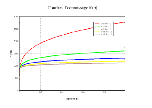
\(R\left(p\right)={\sigma }_{y}+{\sigma }_{y}{\left(\frac{E}{a{\sigma }_{y}}p\right)}^{\frac{1}{n}}\)

The curve representing such a function has the following shape, for various values of n:

The material data is that provided under the keyword factor ECRO_COOK or ECRO_COOK_FO of the operator DEFI_MATERIAU [U4.43.01].

Attention: this work-hardening law is not at all identical to the Ramberg-Osgood law (often used as a hypothesis in simplified analyses in fracture mechanics). The strains-deformations relationship of the Ramberg-Osgood law is:

\(\mathrm{\epsilon }=\frac{\mathrm{\sigma }}{E}+\mathrm{\alpha }\frac{\mathrm{\sigma }}{E}{\left(\frac{\mathrm{\sigma }}{{\mathrm{\sigma }}_{y}}\right)}^{n-1}\) for everything \(\mathrm{\sigma }\).

3.1.4. Relationship VMIS_JOHN_COOK#

The material data is that provided under the keyword factor ECRO_COOK or ECRO_COOK_FO of the operator DEFI_MATERIAU [U4.43.01].

ECRO_COOK =_F (A=A, B=B, C=C, N_PUIS =C, =n, M_PUIS =m, EPSP0 =epsp0, TROOM =troom, TMELT =tmelt,)

The work-hardening curve is written as follows:

\(R\left(p,\dot{p},T\right)=\left(A+B{p}^{n}\right)\left(1+C\mathrm{ln}\left(\frac{\dot{p}}{\dot{{p}_{0}}}\right)\right)\left(1-{\left(\frac{T-{T}_{\mathit{room}}}{{T}_{\mathit{melt}}-{T}_{\mathit{room}}}\right)}^{m}\right)\)

or more concisely:

\(R\left(p,\dot{p},T\right)=\left(A+B{p}^{n}\right)\left(1+C{\dot{p}}^{\ast }\right)\left(1-{{T}^{\ast }}^{m}\right)\)

with \({\dot{p}}^{\ast }=\{\begin{array}{ccc}\frac{\dot{p}}{\dot{{p}_{0}}}& \mathrm{si}& \dot{p}\ge \dot{{p}_{0}}\\ 1& \mathrm{si}& \dot{p}\le \dot{{p}_{0}}\end{array}\) and \({T}^{\ast }=\{\begin{array}{ccc}\frac{T-{T}_{\mathrm{room}}}{{T}_{\mathrm{melt}}-{T}_{\mathrm{room}}}& \mathrm{si}& T\ge {T}_{\mathrm{room}}\\ 0& \mathrm{si}& T\le {T}_{\mathrm{room}}\end{array}\)

3.2. Tangent operator. Option RIGI_MECA_TANG#

The aim of this paragraph is to calculate the tangent operator \({K}_{i-1}\) (calculation option RIGI_MECA_TANG called at the first iteration of a new load increment) from the results known at the previous moment \({t}_{i-1}\).

To do this, if the stress tensor at \({t}_{i-1}\) is on the border of the elasticity domain, we write the condition:

\(\dot{f}=0\)

which should be checked (for the ongoing problem in time) in conjunction with the condition:

\(f=0\)

with:

\(f(\mathrm{\sigma },p)={\mathrm{\sigma }}_{\mathit{eq}}-R(p)\)

If, on the other hand, the stress tensor at \({t}_{i-1}\) is within the domain, \(f<0\), then the tangent operator is the elasticity operator.

The quantities involved in this expression are calculated at the previous moment \({t}_{i-1}\), which are the only ones known at the time of the prediction phase. By calculating the differential:

\(\dot{f}=\frac{\partial f}{\partial \sigma }\dot{\sigma }+\frac{\partial f}{\partial p}\dot{p}=\frac{\partial f}{\partial \sigma }\stackrel{~}{\dot{\sigma }}+\frac{\partial f}{\partial p}\dot{p}\)

because \(\frac{\partial f}{\partial \mathrm{\sigma }}\) is deviating. And so

\(\dot{f}=\frac{\partial f}{\partial \sigma }\left(2\mu \stackrel{~}{\dot{\epsilon }}-2\mu {\dot{\epsilon }}^{P}\right)+\frac{\partial f}{\partial p}\dot{p}=\frac{\partial f}{\partial \sigma }\left(2\mu \dot{\epsilon }-2\mu {\dot{\epsilon }}^{P}\right)+\frac{\partial f}{\partial p}\dot{p}=0\)

With \(\sigma ={\sigma }^{-}=\sigma \left({t}_{\text{i-}1}\right)\), \(\mathrm{\epsilon }={\mathrm{\epsilon }}^{-}=\mathrm{\epsilon }({t}_{i-1})\), \({\mathrm{\epsilon }}^{p}={\mathrm{\epsilon }}^{{p}^{-}}={\mathrm{\epsilon }}^{p}\left({t}_{\text{i-}1}\right)\), and \(p{\text{=p}}^{-}=p\left({t}_{\text{i-}1}\right)\)

Note:

In this expression, the variation of the elastic coefficients with temperature is not taken into account. This is an approximation, with no significant consequences, since this operator is only used to initialize Newton iterations. On the other hand, the dependence of the tangent operator on thermal deformations is well taken into account at the level of the global algorithm [R5.03.01].

When we differentiate the threshold function \(f\) from \(p\), we have

\(\frac{\partial f}{\partial p}=-\frac{dR}{dp}=-{R}^{\text{'}}\left(p\right)\)

We also have \({\dot{\epsilon }}^{p}=\frac{3}{2}\dot{p}\frac{\stackrel{~}{\sigma }}{{\sigma }_{\text{eq}}}\) and \(\frac{\partial f}{\partial \mathrm{\sigma }}=\frac{3}{2}\frac{\stackrel{~}{\mathrm{\sigma }}}{{\sigma }_{\text{eq}}}\), so the expression for \(\dot{f}=0\) can be rewritten

\(\frac{3}{2}\frac{\stackrel{~}{\mathrm{\sigma }}}{{\sigma }_{\text{eq}}}\left(2\mu \dot{\mathrm{\epsilon }}-2\mu \dot{p}\frac{3}{2}\frac{\stackrel{~}{\mathrm{\sigma }}}{{\sigma }_{\text{eq}}}\right)-{R}^{\text{'}}\left(p\right)\dot{p}=0\)

This leads to the following expression for the plastic multiplier:

\(\dot{p}=\frac{\left(3\mu \right)}{{\sigma }_{\text{eq}}}\frac{\left(\stackrel{~}{\mathrm{\sigma }}\text{.}\dot{\stackrel{~}{\mathrm{\epsilon }}}\right)}{3\mu +{R}^{\text{'}}\left(p\right)}\)

therefore

\({\dot{\mathrm{\epsilon }}}^{p}=\{\begin{array}{c}\frac{9\mu }{2}\frac{\left(\stackrel{~}{\mathrm{\sigma }}\text{.}\dot{\stackrel{~}{\mathrm{\epsilon }}}\right)}{3\mu +{R}^{\text{'}}\left(p\right)}\frac{\stackrel{~}{\mathrm{\sigma }}}{{\sigma }_{\text{eq}}^{2}}\text{si}f(\sigma ,p)=0\text{(plasticité)}\\ 0\text{si}f<0\text{(élasticité)}\end{array}\)

The constraint is written

\({\dot{\mathrm{\sigma }}}_{\text{ij}}=3K{\dot{\mathrm{\epsilon }}}_{\text{kk}}{\mathrm{\delta }}_{\text{ij}}+2\mu \left({\dot{\stackrel{~}{\mathrm{\epsilon }}}}_{\text{ij}}-{\dot{\mathrm{\epsilon }}}_{\text{ij}}^{p}\right)\)

Remember that \(2\mu =\frac{E}{1+\nu }\) and \(3K=\frac{E}{1-2\nu }\).

Note:

The information \({\sigma }_{\text{eq}}^{-}-R\left({p}^{-}\right)=0\) is kept in the form of an internal variable \(\xi\) which is 1 in this case and 0 if \({\sigma }_{\text{eq}}^{-}<R\left({p}^{-}\right)\) .

The tangent operator links the virtual deformation vector \({\mathrm{\epsilon }}^{\ast }\) to a virtual stress vector \({\mathrm{\sigma }}^{\ast }\).

The tangent stiffness matrix is written for elastic behavior:

\({\mathrm{\sigma }}^{\ast }=\left(3K\vec{1}\otimes \vec{1}+2\mu \mathrm{P}\right){\mathrm{\epsilon }}^{\ast }\)

and for plastic behavior:

\({\mathrm{\sigma }}^{\ast }=\left(3K\vec{1}\otimes \vec{1}+2\mu \mathrm{P}-{C}_{p}\mathrm{s}\otimes \mathrm{s}\right){\mathrm{\epsilon }}^{\ast }\)

with \(s\) the vector of deviatory constraints associated with \({\sigma }^{-}\) defined by:

\({s}^{T}=\left({\stackrel{~}{s}}_{\text{11}}^{-},{\stackrel{~}{s}}_{\text{22}}^{-},{\stackrel{~}{s}}_{\text{33}}^{-},\sqrt{2}{\stackrel{~}{s}}_{\text{12}}^{-},\sqrt{2}{\stackrel{~}{s}}_{\text{23}}^{-},\sqrt{2}{\stackrel{~}{s}}_{\text{31}}^{-}\right)\)

and:

\({C}_{p}=\xi \frac{{\left(3\mu \right)}^{2}}{{\left({\sigma }_{\text{eq}}\right)}^{2}}\frac{1}{3\mu +{R}^{\text{'}}}\)

\(\xi =\{\begin{array}{c}1\text{si}{\sigma }_{\text{eq}}^{-}-R\left({p}^{-}\right)=0\\ 0\text{sinon}\end{array}\)

In the case of the first loading increment, therefore if the state at the previous instant corresponds to an initial unconstrained state, the tangent operator is identical to the elasticity operator.

3.3. Calculation of constraints and internal variables#

The decomposition of the deformations makes it possible to write:

\(\Delta \varepsilon =\Delta {\varepsilon }^{p}+\Delta ({A}^{-1}\sigma )+\Delta {\varepsilon }^{\text{th}}\)

Or, taking the parts spherical and deviatory:

\(D\tilde{e}={\mathrm{De}}^{p}+D(\frac{\tilde{s}}{\mathrm{2m}})\) because \(\Delta {\tilde{\varepsilon }}^{\text{th}}=0\text{.}\)

\(\text{tr}\Delta \varepsilon =\Delta (\frac{\text{tr}\sigma }{\mathrm{3K}})+\text{tr}\Delta {\varepsilon }^{\text{th}}\) because \(\text{tr}\Delta {\varepsilon }^{p}=0\text{.}\)

By direct implicit discretization of the behavioral relationships for isotropic work hardening, we then obtain:

\(2\mu \Delta \tilde{\varepsilon }-({\tilde{\sigma }}^{-}+\Delta \tilde{\sigma })=\frac{3}{2}2\mu \Delta p\frac{{\tilde{\sigma }}^{-}+\Delta \tilde{\sigma }}{{({\tilde{\sigma }}^{-}+\Delta \tilde{\sigma })}_{\mathrm{eq}}}-2\frac{\mu }{2{\mu }^{-}}{\tilde{\sigma }}^{-}\)

\(\mathrm{tr}\sigma =\frac{\mathrm{3K}}{{\mathrm{3K}}^{-}}\mathrm{tr}{\sigma }^{-}+3K\mathrm{tr}\Delta \varepsilon -3K\mathrm{tr}{\Delta \varepsilon }^{\mathrm{th}}\)

\(\begin{array}{c}{({\sigma }^{-}+\Delta \sigma )}_{\text{eq}}-R({p}^{-}+\Delta p )\le 0\\ \Delta p =0\text{si}{({\sigma }^{-}+\Delta \sigma )}_{\text{eq}}<R({p}^{-}+\Delta p )\\ \Delta p \ge 0\text{si}{({\sigma }^{-}+\Delta \sigma )}_{\text{eq}}=R({p}^{-}+\Delta p )\end{array}\)

To simplify the notations, we define the tensor \({\sigma }^{e}\) such that:

\({\tilde{\sigma }}^{e}=\frac{2\mu }{2{\mu }^{-}}{\tilde{\sigma }}^{-}+2\mu \Delta \tilde{\varepsilon }\) and \(\text{tr}{\sigma }^{e}=\text{tr}\sigma\).

There are two cases:

\({({\sigma }^{-}+\Delta \sigma )}_{\text{eq}}<R({p}^{-}+\Delta p )\)

in this case: \(\Delta p =0\text{soit}\tilde{\sigma }={\tilde{\sigma }}^{-}+\Delta \tilde{\sigma }={\tilde{\sigma }}^{e}\), so: \({({\tilde{\sigma }}^{e})}_{\text{eq}}<R({p}^{-})\)

\({({\sigma }^{-}+\Delta \sigma )}_{\text{eq}}=R({p}^{-}+\Delta p )\)

in this case: \(\Delta p \ge 0\) so: \({({\tilde{\sigma }}^{e})}_{\text{eq}}\ge R({p}^{-})\)

The resolution algorithm is deduced from this:

if \({\tilde{\sigma }}_{\text{eq}}^{e}\le R({p}^{-})\) then \(\Delta p=0\text{soit}\tilde{\sigma }={\tilde{\sigma }}^{-}+\Delta \tilde{\sigma }={\tilde{\sigma }}^{e}\)
if \({\tilde{\sigma }}_{\text{eq}}^{e}>R({p}^{-})\)

so we have to solve: \(\tilde{{\sigma }^{e}}=\tilde{{\sigma }^{-}}+\Delta \tilde{\sigma }+\frac{3}{2}2\mu \Delta p\frac{{\tilde{\sigma }}^{-}+\Delta \tilde{\sigma }}{{({\sigma }^{-}+\Delta \sigma )}_{\mathrm{eq}}}\)

so by factorizing \({\tilde{\sigma }}^{-}+\Delta \tilde{\sigma }\) and taking the equivalent Von Mises value:

\({\sigma }_{\text{eq}}^{e}=(1+\frac{3}{2}\frac{2\mu \Delta p }{{({\sigma }^{-}+\Delta \sigma )}_{\text{eq}}}){({\sigma }^{-}+\Delta \sigma )}_{\text{eq}}\)

either:

\({\sigma }_{\text{eq}}^{e}=R({p}^{-}+\Delta p )+3\mu \Delta p\)

car: \({\sigma }_{\text{eq}}={({\sigma }^{-}+\Delta \sigma )}_{\text{eq}}=R(\overline{p}+\Delta p )\)

It is a scalar equation in \(\Delta p\), linear or not according to \(R(p)\). \(\Delta p\) is calculated as follows:

in the case where the work hardening is linear (relationship VMIS_ISOT_LINE), we obtain directly:

\(\Delta p =\frac{{\sigma }_{\mathrm{eq}}^{e}-{\sigma }_{y}-R\text{'}{p}^{-}}{R\text{'}+3\mu }\) \(R\text{'}=\frac{E{E}_{T}}{E-{E}_{T}}\) with

in the case where work-hardening is given by a tensile curve that is refined by pieces, (relationship VMIS_ISOT_TRAC), we take advantage of piecewise linearity to determine exactly \(\Delta p\) (see § Annexe 1);
in the case of work hardening defined by a power law (relationship VMIS_ISOT_PUIS), \(\Delta p\) is a solution of the non-linear equation: \(R({p}^{-}+\Delta p )+3\mu \Delta p -{\sigma }_{\text{eq}}^{e}=0\). This equation is solved by an iterative method (secant algorithm). In the vicinity of the origin, we linearize \(R(p)\), because the derivative \({R}^{\text{'}}=\frac{E}{\text{an}}{(\frac{E}{a{\sigma }_{y}}p)}^{\frac{1}{n}-1}\) is infinite in \(p=0\). So if \(p<{p}_{0}\), we replace \(R(p)\) with \({R}^{\text{lin}}(p)={\sigma }_{y}+\frac{p}{{p}_{0}}(R({p}_{0})-{\sigma }_{y})\), which avoids the search for a numerically almost zero solution. In practice, we choose \({p}_{0}={\text{10}}^{-\text{10}}\).

Once \(\Delta p\) is determined, \(\sigma\) is calculated by:

\({\tilde{\sigma }}^{-}+\Delta \tilde{\sigma }=\frac{{\sigma }_{\text{eq}}^{e}-3\mu \Delta p }{{\sigma }_{\text{eq}}^{e}}\text{.}{\tilde{\sigma }}^{e}\)

and

\(\text{tr}({\sigma }^{-}+\Delta \sigma )=\text{tr}{\sigma }^{e}\).

Options RAPH_MECA and FULL_MECA both perform the previous calculation, which explains the calculation of \(R({u}_{i}^{n})\). Note that in reality, \(R({u}_{i}^{n})={Q}^{T}{\sigma }_{i}^{n}\) where \({\sigma }_{i}^{n}\) is calculated not according to \({u}_{i}^{n}\), but to \({\sigma }_{i-1}\text{et}{\Delta u }_{i}^{n}\).

Note:

Special case of plane stresses.

The Von Mises model with isotropic work hardening (VMIS_ISOT_LINE, VMIS_ISOT_PUIS or VMIS_ISOT_TRAC) is also available in plane constraints, i.e. for models C_PLAN, DKT, COQUE_3D, COQUE_AXIS, COQUE_D_PLAN,, COQUE_C_PLAN, or,, or) TUYAU TUYAU_6M ..

In this case, the system to be solved includes an additional equation. This calculation is detailed in Appendix 2.

3.4. Tangent operator. Option FULL_MECA#

Option FULL_MECA allows you to calculate the tangent matrix \({K}_{i}^{n}\) at each iteration. The tangent operator that is used to construct it is calculated directly on the previous discretized system (we note for simplicity: \(\tilde{\sigma }=\tilde{{\sigma }^{-}}+\Delta \tilde{\sigma },p={p}^{-}+\Delta p\)) and we write the expressions only in the isothermal case.

If the stress tensor is on the domain border, \(f=0\) then we have, differentiating the expression from the law of normality in \(\tilde{\sigma }=\tilde{{\sigma }^{-}}+\Delta \tilde{\sigma }\):

\(2\mu {\delta \varepsilon }^{p}=2\mu \delta \tilde{\varepsilon }-\delta \tilde{\sigma }=\frac{3}{2}2\mu (\deltap \frac{\tilde{\sigma }}{{\sigma }_{\text{eq}}}+\Delta p \frac{\delta \tilde{\sigma }}{{\sigma }_{\text{eq}}}-\frac{3}{2}\Delta p \frac{\tilde{\sigma }:d\tilde{\sigma }}{{\sigma }_{{\text{eq}}^{3}}}\text{.}\tilde{\sigma })\)

where \({\delta \varepsilon }^{p},\delta \tilde{\varepsilon },\delta \tilde{\sigma }\) represent infinitesimal increases around the solution of the incremental elastoplastic problem obtained previously.

Like:

\(\frac{3}{2}\frac{\tilde{\sigma }:d\tilde{\sigma }}{{\sigma }_{\text{eq}}}={R}^{\text{'}}(p)\mathrm{dp}\)

by performing the tensor product of the first equation by \(\tilde{\sigma }\) we have:

\(2\mu \tilde{\sigma }:\delta \tilde{\varepsilon }-\tilde{\sigma }:\delta \tilde{\sigma }=2\mu \deltap \text{.}{\sigma }_{\text{eq}}\)

by eliminating \(\deltap\) from the last two equations:

\(\tilde{\sigma }:\delta \tilde{\sigma }=\frac{2\mu \tilde{\sigma }:\delta \tilde{\varepsilon }}{1+\frac{3\mu }{{R}^{\text{'}}(p)}}\).

If, on the other hand, if the stress tensor is inside the domain, \(f<0\), then the tangent operator is the elasticity operator.

Expressing \(\deltap\) and \(\tilde{\sigma }:\delta \tilde{\sigma }\) in the first equation gives:

\(2\mu \delta \tilde{\varepsilon }-\delta \tilde{\sigma }=\frac{3\mu \Delta p }{{\sigma }_{\text{eq}}}\delta \tilde{\sigma }+{C}_{p}\text{.}{(\tilde{\sigma }:\delta \tilde{\varepsilon })}_{+}\tilde{\sigma },\)

with:

\({C}_{p}=\frac{9{\mu }^{2}}{{\sigma }_{\mathrm{eq}}^{2}}(1-\frac{{R}^{\text{'}}(p)\Delta p}{{\sigma }_{\text{eq}}})\frac{1}{{R}^{\text{'}}(p)+3\mu }\)

The positive part \({(\tilde{\sigma }:\delta \tilde{\varepsilon })}_{+}\) allows you to combine the two conditions into a single equation:

be \(f<0\), which implies \(\Delta p =0\)
be \(f=0\)

We then obtain:

\(\delta \tilde{\sigma }=\frac{2\mu }{a}\delta \tilde{\varepsilon }-\frac{{C}_{p}}{a}{(\tilde{\sigma }:\delta \tilde{\varepsilon })}_{+}\tilde{\sigma }\)

by asking:

\(a=1+\frac{3\mu \Delta p }{R(p+\Delta p )}\)

The tangent operator links the virtual deformation vector \({\varepsilon }^{\ast }\) to a virtual stress vector \({\sigma }^{\ast }\).

The tangent stiffness matrix is written for elastic behavior:

\({\sigma }^{\ast }=(K\overrightarrow{1}\otimes \overrightarrow{1}+2\mup ){\varepsilon }^{\ast }\)

and for plastic behavior:

\({\sigma }^{\ast }=(K\overrightarrow{1}\otimes \overrightarrow{1}+\frac{2\mu }{a}P-\frac{{C}_{p}}{a}s\otimes s){\varepsilon }^{\ast }\)

with \(s\) the vector of deviatory constraints associated with \({\sigma }^{-}\) defined by:

\({s}^{T}=({\tilde{\sigma }}_{\text{11}}^{-},{\tilde{\sigma }}_{\text{22}}^{-},{\tilde{\sigma }}_{\text{33}}^{-},\sqrt{2}{\tilde{\sigma }}_{\text{12}}^{-},\sqrt{2}{\tilde{\sigma }}_{\text{23}}^{-},\sqrt{2}{\tilde{\sigma }}_{\text{31}}^{-})\)

and:

\(\xi =\{\begin{array}{c}1\text{si}\Delta \varepsilon \text{conduit à une plastification}\text{et}\tilde{\sigma }\text{.}\Delta \tilde{\varepsilon }\ge 0\\ 0\text{sinon}\end{array}\)

It can be seen that the operator tangent to the system resulting from the implicit discretization differs from the operator tangent to the speed problem (RIGI_MECA_TANG). It can be found by doing: \(\Delta p =0\) in the expressions in \({C}_{p}\) and \(a\).

3.5. Internal behavior variables VMIS_ISOT_LINE, VMIS_ISOT_PUIS,, VMIS_ISOT_TRAC, and VMIS_JOHN_COOK#

Behavioral relationships VMIS_ISOT_LINE, VMIS_ISOT_PUIS, and VMIS_ISOT_TRAC produce two internal variables:

\(p\) cumulative equivalent plastic deformation,
and \(\chi\) indicator of plasticity at the moment in question (useful for calculating the tangent operator).

VMIS_JOHN_COOK uses two internal variables in addition to the previous two:

\(\dot{{p}^{\mathrm{-}}}\) cumulative equivalent plastic deformation rate at the moment minus,
and \(\Delta {t}^{-}\) the time step increment at the moment minus.