2. One-dimensional viscoelastic stress-strain relationship

The equivalent linear model is based on the Kelvin-Voigt viscoelastic rheological model. The latter, represented in, consists in parallel of a linear spring and a linear damper representing an internal resistance to deformation.

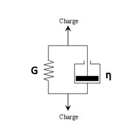
Figure 2-1: Representation of the Kelvin-Voigt rheological model.

The constitutive relationship of this rheological model is as follows:

(2.1)\[ {\ sigma} _ {\ mathrm {xz}} =G\ gamma +H\ frac {\ partial\ gamma} {\ partial t} =G\ gamma +H\ dot {\ gamma}\]

with \({\sigma }_{\mathrm{xz}}\) shear stress, \(\gamma\) the distortion (equal to \(2{\epsilon }_{\mathit{xz}}\)), \(G\) the shear modulus and \(H\) the viscosity modulus. The dot represents the time derivative.

In the case of a one-dimensional soil column, by noting \(u(z,t)\) the horizontal displacement at a given depth \(z\) and at a given time \(t\), the distortion and its temporal drift are defined from the displacement field \(u(z,t)\):

(2.2)\[ \ gamma =\ frac {\ partial u (z, t)} {\ partial z}\]

And its time derivative:

\[\]

: label: eq-4

dot {gamma} =frac {partialgamma (z, t)} {partial t} =frac {{partial} ^ {2} u (z, t)}} {partial zpartial t}

In the case of harmonic loading \(u(z,t)=U(z){e}^{i\omega t}\), the distortion is written as:

\[\]

: label: eq-5

gamma (z, t) =frac {partial u (z, t)} {partial z} =frac {mathit {dU} (z)} {mathit {dz}} {e}} {e}} {e} ^ {e} ^ {e} ^ {e} ^ {e} ^ {e} ^ {e} ^ {e} ^ {e} ^ {e} ^ {e} ^ {e} ^ {e} ^ {e} ^ {e} ^ {e} ^ {e} ^ {iomega t} ^ {iomega t} =mathrm {gamma} (z) {e} ^ {iomega t}

And its time derivative:

(2.3)\[ \ dot {\ gamma} (z, t) =i\ omega\ gamma (z, t)\]

with \(U(z)\) and \(\mathrm{\Gamma }(z)\) respectively the magnitude of displacement and distortion.

The stress-strain relationship constituting the Kelvin-Voigt model is then defined:

(2.4)\[ {\ sigma} _ {\ mathrm {xz}} (z, t)} (z, t) =G\ gamma +H\ dot {\ gamma} =G (1+i\ eta\ omega)\ gamma (z, t)\ gamma (z, t) = {G}} = {G} ^ {\ ast}\ gamma (z, t)\]

with \({G}^{\text{*}}\) complex shear modulus \({G}^{\ast }=(G+i\eta \omega )\); the loss factor here is equal to \(\eta \omega\).

During symmetric cyclic loading, the soil response presents cycles or hysteresis loops in the stress-strain plane (see).

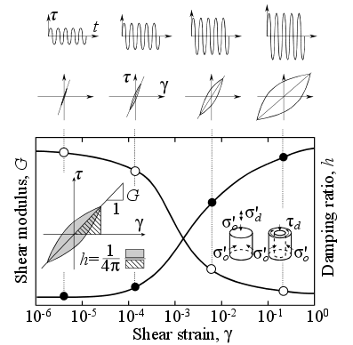
Figure2-2. Response of a soil to symmetric cyclic loading, \({\sigma }_{\mathrm{xz}}\) the shear stress, \(\gamma\) the distortion, \(D\) the damping [4].

These loops represent the quantity of deformation energy dissipated by the ground during loading. This energy can be quantified by defining the reduced damping coefficient \(D\) (see the) of the ground by the following relationship:

(2.5)\[ D=\ frac {{W} _ {d}}} {4\ mathrm {\ pi} {W} _ {s}}\]

where \({W}_{d}\) represents the energy dissipated in a complete loading cycle (equal to the internal area formed by the stress-strain loop, in gray on the), and \({W}_{s}\) the elastic energy stored by the ground during loading for the distortion level \({\mathrm{\gamma }}_{c}\) (lower triangle, shaded on the).

These two energies are calculated in the case of harmonic loading \(\gamma (t)={\gamma }_{c}{e}^{i\omega t}\) with the Kelvin-Voigt model:

(2.6)\[ {W} _ {d} =\ underset {{{\ mathrm {\ mathrm {\ sigma}}} _ {\ mathit {xz}}} {\ oint} {\ mathrm {\ sigma}}} _ {\ mathit {xz}} _ {\ mathit {xz}}} _ {\ mathit {xz}}} _ {\ mathit {xz}}} _ {\ mathit {xz}}} d\ mathrm {\ gamma}} =\ underset {t} {\ oint} {\ oint} {\ mathrm {\ sigma}} {\ mathrc}} _ {\ mathrm {\ sigma}}} _ {\ mathrm {\ sigma}}} _ {\ mathrm {\ sigma}}} _ m {\ pi}} {\ mathrm {\ omega}}}} {\ oint}} {\ oint}}\ mathrm {\ Re}} [{\ mathrm {\ sigma}} _ {\ mathit {xz}}]\ mathrm {\ omega}}]\ mathrm {\ omega}}]\ mathrit {xz}}]\ mathrm {\ Re}}]\ mathrm {\ Re}} [\ frac {d\ mathrm {\ gamma}}} {\ mathit {dt}}]\ mathit {dt}}]\ mathrit {dt}}]\ mathrit {dt}}]\ mathrm {\ Re}}}\ mathrm {\ Re}} [\ frac {d m {\ pi}\ mathrm {\ eta}\ mathrm {\ omega} {\ mathrm {\ gamma}} _ {c} ^ {2}\]

And:

(2.7)\[ {W} _ {s} =\ frac {1} {2} {2} {\ mathrm {\ tau}} _ {c} {\ mathrm {\ gamma}} _ {c} =\ frac {1} {2} {2} G {\ mathrm {\ tau}}} _ {c} ^ {2} =\ frac {1} {2} {2}\]

For the Kelvin-Voigt viscoelastic model, the energy dissipated during a loading cycle therefore depends on the stress frequency. However, experience shows that for soils, the energy dissipated during shearing is almost independent of the deformation rate. Damping results essentially from irreversible plastic deformations at the grain level. Damping in the ground is more hysteretic than viscous [5]. The Kelvin-Voigt model is thus modified so that the dissipative properties are equivalent to the real material.