6. Implementation of the equivalent linear in code_aster#

The command DEFI_SOL_EQUI [U4.84.31] makes it possible to calculate the response of a one-dimensional ground column to seismic stress with the equivalent linear model (Schnabel or Lysmer formulation) in convolution or deconvolution.

The method for solving the equivalent linear model is an iterative procedure, where equivalent linear characteristics are evaluated at each iteration for each layer on the basis of the degradation curves of the shear module \(G\) and the increase in hysteretic damping.

The command outputs time signals, Oscillator Response Spectra (SRO), temporal deformations and stresses at various depths, and degraded soil properties in accordance with the calculated shear strain levels.

The user must enter the command:

A table giving the \(G/{G}_{\mathit{max}}\) ratio as a function of Gamma,
A table showing the reduced damping of material \(D\) as a function of Gamma,
A table describing the initial material characteristics of the various layers (Young’s modulus E, density RHO, fish ratio NU, hysteretic damping AMOR_HYST, possibly the value of \({({N}_{1})}_{60}\) N1 for obtaining the parameters of the Byrne model). Hysteretic damping is equal to twice critical damping \(\mathit{AH}=2D\) (see justification in § 4.2.).
The 2D/3D mesh of the column respecting a \({L}_{\mathit{max}}<\frac{{V}_{s}}{8{f}_{\mathit{coupure}}}\) mesh size,
A time signal (one component or three components) imposed in open field conditions or on an outcrop rock.

6.1. Boundary conditions of the model#

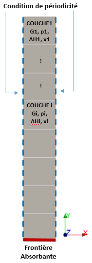
The underlying model is a 2D soil column with the following boundary conditions: Right and left edges of the column: periodicity condition. This means that the movements of the nodes on the left and right faces facing each other are made equal. Infinite horizontal layers are thus modelled. Bottom of the column: assignment of an absorbent border element (cf. [] Absorbing border elements). The substratum is thus modelled as an infinite medium. Depending on the coefficient given to the element, part of the waves is reflected at the interface, while the other part is dissipated (by radiative damping). The absorbent border adopts the D_ PLAN_ABSO modeling. The other elements adopt the D_ PLAN modeling.

The underlying model is a 3D ground column with the following boundary conditions: Edges lateral:periodicity condition, applied as follows: equal displacement of the nodes from two faces facing each other; equal displacement of the nodes facing each other; equal displacement of the nodes facing each other; equal displacement of the nodes facing each other of the faces facing each other; equal displacement of the nodes facing each other of the edges 1 and 2 in one of the previously chosen faces. Infinite horizontal layers are thus modelled. Bottom of the column: assignment of an absorbent border element (cf. [] Absorbing border elements). The substratum is thus modelled as an infinite medium. Depending on the coefficient given to the element, part of the waves is reflected at the interface, while the other part is dissipated (by radiative damping). The absorbent border adopts 3D modeling_ ABSO. The other elements adopt 3D modeling.

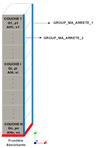
6.2. Equivalent linear model formulations#

The command models damping by hysteretic damping (operator DEFI_MATERIAU keyword AMOR_HYST). From the Young’s modulus \(E\) and the hysteretic damping \(\mathrm{AH}\) specified in DEFI_MATERIAU, code_aster builds the complex module \({E}^{\ast }\) according to the equation:

\[\]

: label: eq-28

{E} ^ {ast} =E (1+mathrm {I.ah})

The construction of the complex module therefore corresponds to the Schnabel formulation described in § 4.1 si \(\mathit{AH}=\mathrm{2D}\). This is why it is necessary to specify \(2{D}_{\mathrm{min}}\) as the initial value in the floor table.

However, if the user has chosen the Lysmer formulation, the command calculates, based on material data \(E\) and \(\mathit{AH}\), a module \({E}_{1}\) and an equivalent damping \({\mathit{AH}}_{1}\) such that the Lysmer formulation is found:

(6.1)#\[ {E} _ {1}\ left (1+i {\ mathit {AH}}} _ {1}\ right) =E\ left (\ left (1-\ frac {{\ mathit {AH}}} ^ {2}}} {2}} {2}\ right) +\ mathit {II}\ right) +\ mathit {ii}\ right) +\ mathit {ii}\ right) = E\ left (\ left (1-\ frac {{\ mathit {AH}}} ^ {AH}} ^ {2}}\ right) +\ mathit {ii}\ right) +\ mathit {ii}\ right) +\ mathit {ii}\ right}\ mathit {AH}}\ right}} {4}}\ right)\]

By equating the parts real and imaginary of two previous equations, the following relationships are obtained:

\[\]

: label: eq-30

{E} _ {1} =Eleft (1-frac {{mathit {AH}} ^ {2}} {2}} {2}right)

textrm {and}

{mathit {AH}} _ {1} =mathit {AH}sqrt {1-frac {{mathit {AH}}} ^ {2}}} {2}}} {2}} {2}} {4}}

In this form, the equivalent linear method does not have a dependence of damping on frequency.

6.3. Resolution method#

The procedure for resolving the order issue is the following iterative procedure:

Assignment of the initial shear and damping modules (\(G={G}_{\mathrm{max}}\), \(D={D}_{\mathrm{min}}\)) at each discretization point in the soil column.
Calculation of complex shear modules according to the formulation of the equivalent linear model chosen (Schnabel or Lysmer) using \(G\) and \(D\) filled in.
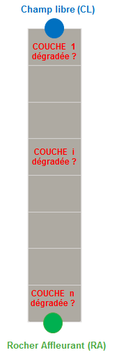
Calculation of the harmonic response of the ground column: excitation by a unit white noise at the base of the column (edge noted RA): \({A}_{\mathit{RA}}^{\mathit{harm}}=1\) on the selected frequency band DYNA_VIBRA, TYPE_CALCUL = “HARM”.
The harmonic accelerations at each depth are recovered and the transfer functions between the outlying rock RA, and the free field CL, and the various layers \(i\) are calculated.

Noting \({A}^{\mathit{harm}}{}_{i}\), the harmonic acceleration of layer \(i\), it comes from:

\(\mathit{Fonction}\mathit{de}{\mathit{transfert}}_{\mathit{CL}/\mathit{RA}}=\frac{1+{A}^{\mathit{harm}}{}_{\mathit{CL}}}{{A}^{\mathit{harm}}{}_{\mathit{RA}}}=\frac{1+{A}^{\mathit{harm}}{}_{\mathit{CL}}}{1}\) \(\mathit{Fonction}\mathit{de}{\mathit{transfert}}_{i/\mathit{RA}}=\frac{1+{A}^{\mathit{harm}}{}_{i}}{1}\) Since the calculation is in relative motion (CHARGEMENT =” MONO_APPUI “), the training movement should be added to the harmonic accelerations of each layer. Here, the training motion is \(1\), which explains the numerator expression for the transfer function \(1+{A}^{\mathit{harm}}{}_{\mathit{CL}}\). If the calculation is in absolute motion (CHARGEMENT =” ONDE_PLANE “), the transfer functions are reduced to the harmonic response of each layer.

Calculation of the Fourier transform (FFT) of the input signal (frequency transition).
Convolution/deconvolution of the input signal in the column (Multiplication of the transfer functions by the FFT of the input signal). If the imposed signal is a rock flush with RA, it is convoluted using the transfer functions defined above. If the imposed signal is in free field CL, the corresponding flush rock signal is calculated with the RA/CL transfer function for CHARGEMENT =” MONO_APPUI “:

\(\mathit{Fonction}\mathit{de}{\mathit{transfert}}_{\mathit{RA}/\mathit{CL}}=\frac{1}{1+{A}^{\mathit{harm}}{}_{\mathit{CL}}}\)

Calculation of deformations \(\mathrm{\gamma }(f)\) in each layer.

For the case of a 1D — 3 components modeling, the value of the deformations \({\mathrm{\epsilon }}_{\mathit{xy}}(f)\), \({\mathrm{\epsilon }}_{\mathit{yz}}(f)\) and \({\mathrm{\epsilon }}_{\mathit{yy}}(f)\) are recovered in order to calculate the equivalent deformation.

Calculation of inverse Fourier transforms \(\mathrm{\gamma }(t)\) (temporal feedback).

For the case of a 1D — 3 component modeling, the value of \({\mathrm{\epsilon }}_{d}(t)\) is obtained from the deformations \({\mathrm{\epsilon }}_{\mathit{xy}}(t)\), \({\mathrm{\epsilon }}_{\mathit{yz}}(t)\) and \({\mathrm{\epsilon }}_{\mathit{yy}}(t)\) by the following expression:

\({\mathrm{\epsilon }}_{d}=\frac{2}{3}\sqrt{{\mathrm{\epsilon }}_{\mathit{yy}}^{2}+3{\mathrm{\epsilon }}_{\mathit{xy}}^{2}+3{\mathrm{\epsilon }}_{\mathit{yz}}^{2}}\)

The value of \(\mathrm{\gamma }(t)\) is then calculated from \({\mathrm{\epsilon }}_{d}(t)\).

Calculation in each layer of the effective shear deformation defined as:

\({\mathrm{\gamma }}_{\mathit{effective}}=\mathrm{\chi }\mathrm{.}{\mathrm{\gamma }}_{\mathit{max}}\)

with \({\gamma }_{\mathrm{max}}\) maximum shear deformation calculated in the layer and \(\chi\) effective deformation weighting coefficient (COEF_GAMMA, by default is equal to \(\mathrm{0,65}\), see §7).

Evaluation for each layer of the shear modulus and the damping corresponding to \({\mathrm{\gamma }}_{\mathit{effective}}\) on the corresponding \(G/{G}_{\mathit{max}}\) -Gamma and \(D\) -Gamma curves.

In the case of simplified modeling of water pressure using the Byrne model, the following formula is used for the evaluation of the shear modulus:

\(G/{G}_{\mathit{max}}({\mathrm{\gamma }}_{\mathit{effective}})\mathrm{.}{(1-{\mathrm{\chi }}_{\mathit{ru}}{r}_{\mathit{umax}})}^{\mathrm{0,5}}\)

where \({r}_{\mathit{umax}}\) represents the maximum of the evolution history of \({r}_{u}\) and \({\mathrm{\chi }}_{\mathit{ru}}\) is a weighting coefficient that makes it possible to modulate the impact of \({r}_{\mathit{umax}}\) on the effective deformation (COEF_KSI, by default is equal to \(\mathrm{0,667}\)). We therefore multiply the value of \(G/{G}_{\mathit{max}}\) evaluated at \({\mathrm{\gamma }}_{\mathit{effective}}\) by the expression taking into account the rise in water pressure.

Damping is evaluated with the expression of \({\mathrm{\gamma }}_{\mathit{effective}}\) without taking into account water pressure.

If \(∣\frac{{G}_{k+1}-{G}_{k}}{{G}_{k}}∣>\theta\) (with \(\theta =5\text{\%}\) by default (RESI_RELA)), go back to step 2 with the new \({G}_{k+1}\) modules for each layer.
If convergence is reached, post-processing takes place. The command calculates accelerations, stresses, deformations, in time (FFT inverse), and SRO for each layer. The degraded properties of the column are also given.