3. Validation of the model on a few examples#
Applications on cylinders and plates are presented here. The first in fact treats a one-dimensional case in thickness and makes it possible to evaluate the effect of curvature terms, especially in the second member of the equations. The others make it possible to judge the capacity of the model to deal with the case of discontinuous thermal loads, by reference to 3D solutions.
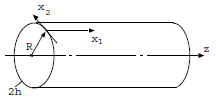
3.1. The infinite cylinder subjected to a uniform internal flow#
We consider an infinite cylinder (radius \(R\), thickness \(\mathrm{2h}\)), subject to a uniform flow inside: \({\varphi }_{i}\), and to an exchange condition in external skin \({\lambda }^{+}(T-{T}_{\mathrm{ext}})={\lambda }^{+}T-{\varphi }_{{e}^{-}}\).
The transverse conductivity coefficient is denoted \(K\).
The analytical solution to this 1D axisymmetric problem is:
\(T({x}_{3})=\stackrel{ˆ}{{T}_{1}}+\stackrel{ˆ}{{T}_{0}}\mathrm{ln}(1+{x}_{3}/R)\)
\(-{KT}_{\mathrm{,3}}={\varphi }_{i}>0\)
\({\lambda }^{\text{+}}T-{\varphi }_{e}=-{KT}_{\mathrm{,3}}\)
Figure: 3.1-a
with:
\(\stackrel{ˆ}{{T}_{0}}=-\frac{R{\varphi }_{i}}{K}(1-\frac{h}{R})\)
\(\stackrel{ˆ}{{T}_{1}}=\frac{R{\varphi }_{i}}{K}(1-\frac{h}{R})\mathrm{ln}(1+\frac{h}{R})+({\varphi }_{i}\frac{1-h/R}{1+h/R}+{\varphi }_{e})\mathrm{.}\frac{1}{{\lambda }^{+}}\)
A development limited to the 2nd order in \({x}_{3}/R\) is:
\(T({x}_{3})\approx \frac{{\varphi }^{+}+{\varphi }^{-}}{{\lambda }^{+}}-\frac{2{\varphi }_{i}}{{\lambda }^{+}}\mathrm{.}\frac{h}{R}\left[1-\frac{h}{R}-\frac{{\lambda }^{+}R}{\mathrm{2k}}(1-\frac{\mathrm{3h}}{\mathrm{2R}})\right]-{\varphi }_{i}\frac{h}{K}(1-\frac{h}{R})(\frac{{x}_{3}}{h}-\frac{{x}_{3}^{2}}{{\mathrm{2h}}^{2}}\mathrm{.}\frac{h}{R})+\mathrm{...}\)
Now let’s use the 3-field model \(T=({T}_{\mathrm{1,}}{T}_{\mathrm{2,}}{T}_{3})\) defined in [§ 2.3.2]. Because of the independence in \({\mathrm{x}}_{1}\) and \({\mathrm{x}}_{2}\) of the solution, we are back to the resolution of: \(BT=C\).
For representation \(T({x}_{3})={T}_{1}+{T}_{2}\frac{{x}_{3}}{h}+\frac{3}{2}\mathrm{.}{T}_{3}(\frac{{x}_{3}^{2}}{{h}^{2}}-\frac{1}{3})\), we have:
\(B=\frac{\mathrm{2K}}{h}(\begin{array}{ccc}0& 0& 0\\ 0& 1& h/R\\ 0& h/R& 3\end{array})+{\lambda }^{+}(1+\frac{h}{R})(\begin{array}{ccc}1& 1& 1\\ 1& 1& 1\\ 1& 1& 1\end{array})\)
\(C={\varphi }_{i}(1-\frac{h}{R})(\begin{array}{}1\\ -1\\ 1\end{array})+{\varphi }_{e}(1+\frac{h}{R})(\begin{array}{}1\\ 1\\ 1\end{array})\) for the second member.
In the case where we neglect the intervention of curvature in the metric, we remove the terms in \(\frac{h}{R}\) in the previous expressions.
The solution is, if we completely overlook curvature \((1\gg \frac{h}{R})\):
\(T({x}_{3})=\frac{{\varphi }_{e}+{\varphi }_{i}}{{\lambda }^{+}}+\frac{{\varphi }_{i}\mathrm{.}h}{K}(1-\frac{{x}_{3}}{h})\) i.e. the solution of the plane « wall ».
If we take into account the curvature in the second member as well as in the terms of trade \({\lambda }^{+}\) (real areas of application of the flows):
\(T({x}_{3})=\frac{{\varphi }_{i}+{\varphi }_{e}}{{\lambda }^{+}}-\frac{2{\varphi }_{i}}{{\lambda }^{+}}\mathrm{.}\frac{h}{R}\left[1-\frac{h}{R}-\frac{{\lambda }^{+}R}{\mathrm{2k}}(1-\frac{h}{R})\right]-{\varphi }_{i}\frac{h}{K}(1-\frac{h}{R})\mathrm{.}\frac{{x}_{3}}{h}+0\)
We find the analytical solution developed in the 1st order in \({x}_{3}/R\). Taking curvature into account in the conductivity terms in \(B\) would occur at the level of the terms in \({({x}_{3}/R)}^{2}\).
3.2. The infinite plate under a pair of antisymmetric flows#
Let’s go back to the case of the infinite plate subjected on its \({x}_{2}<0\) half to a pair of balanced \(({\varphi }^{+}=\varphi ,{\varphi }^{-}=-\varphi )\) constant flows, and adiabatic on the other half \({x}_{2}>0\).
The antisymmetry of the load requires that: \(T({x}_{\mathrm{1,}}{x}_{2}\mathrm{,0})=0\). We can also show that \(T\) is linear in thickness in \({x}_{2}=-\infty ,\mathrm{0,}+\infty\).
The equations [éq 2.3.2-2] here are reduced to:
\(-\mathrm{2kh}(\begin{array}{ccc}1& 0& 0\\ 0& 1/3& 0\\ 0& 0& 1/5\end{array})(\begin{array}{}{T}_{1}\\ {T}_{2}\\ {T}_{3}\end{array})+\frac{\mathrm{2K}}{h}(\begin{array}{ccc}0& 0& 0\\ 0& 1& 0\\ 0& 0& 3\end{array})(\begin{array}{}{T}_{1}\\ {T}_{2}\\ {T}_{3}\end{array})=\varphi (\begin{array}{}0\\ 2\\ 0\end{array})\)
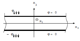
Figure: 3.2-a
Since derivatives \({T}_{i\mathrm{,2}}\) cancel out infinitely, \({\mathrm{T}}_{1}\) and \({\mathrm{T}}_{3}\) are identically zero everywhere. It remains to be determined \({T}_{2}\) (depending only on \({x}_{2}\)) such that:
\(-{T}_{2}^{\text{'}\text{'}}+\frac{\mathrm{3K}}{{\text{kh}}^{2}}\text{.}{T}_{2}=\frac{3\varphi }{\text{kh}}\) whose solution is of the form:
\(\{\begin{array}{}{T}_{2}({x}_{2})=a{e}^{\sqrt{\mathrm{3K}/k}\mathrm{.}{x}_{2}/h}+\frac{\varphi h}{K}\text{si}{x}_{2}<0\text{,}\\ {T}_{2}({x}_{2})=b{e}^{-\sqrt{\mathrm{3K}/k}\mathrm{.}{x}_{2}/h}\text{si}{x}_{2}>0\text{,}\end{array}\)
The continuity of \({T}_{2}\) and \({T}_{2}^{\text{'}}\) in \(0\) gives:
\(\{\begin{array}{}{T}_{2}({x}_{2})=\frac{\varphi h}{K}(2-{e}^{\sqrt{\mathrm{3K}/k}\mathrm{.}{x}_{2}/h})\text{si}{x}_{2}\le 0\text{}\\ {T}_{2}({x}_{2})=\frac{\varphi h}{K}{e}^{-\sqrt{\mathrm{3K}/k}\mathrm{.}{x}_{2}/h}\text{si}{x}_{2}\ge 0\text{}\end{array}\)
After changing the variables \({T}^{m},{T}^{s},{T}^{i}\), we find:
\({T}^{m}({x}_{2})=0\text{;}{T}^{s}({x}_{2})={T}_{2}({x}_{2})\text{;}{T}^{i}({x}_{2})=-{T}_{2}({x}_{2})\)
The temperature of the plate, calculated in the framework of this model, is therefore linear in thickness and is expressed with \({\mathrm{T}}^{\mathrm{m}}({\mathrm{x}}_{2})\) or \({\mathrm{T}}^{\mathrm{s}}({\mathrm{x}}_{2})\) and \({\mathrm{T}}^{\mathrm{i}}({\mathrm{x}}_{2})\) by:
\(T({x}_{\mathrm{1,}}{x}_{\mathrm{2,}}{x}_{3})={T}_{2}({x}_{2})\mathrm{.}\frac{{x}_{3}}{h}={T}^{s}({x}_{2})\mathrm{.}\frac{{x}_{3}}{\mathrm{2h}}(1+{x}_{3}/h)-{T}^{i}({x}_{2})\mathrm{.}\frac{{x}_{3}}{\mathrm{2h}}(1-{x}_{3}/h)\)
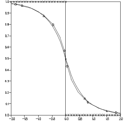
The [Figure 3.2-a] makes it possible to compare the temperatures in the upper skin \(({x}_{3}=+h)\) of the plate under a normalized external flow (\(\varphi \mathrm{=}K\mathrm{/}h\) with \(k\mathrm{=}K\mathrm{=}\mathrm{1,}h\mathrm{=}1\)), obtained by a 3D numerical calculation (Code Aster), the shell model, and the asymptotic limit model (with the discontinuity observed in [§2.2]).
We note the good capacity of the model to describe the boundary layer appearing in the vicinity of an external flow discontinuity.
Homogeneous plate
|
|
Figure 3.2-b: Comparative temperature in the upper skin of the plate subjected to antisymmetric flows.
3.3. The infinite plate under a pair of symmetric flows#
In the previous example, load antisymmetry caused even terms to be null in \({x}_{3}({T}_{1}={T}_{3}=0)\). We now treat another case of loading, symmetric, (with respect to \({x}_{3}=0\)) making it possible to judge the effect of the term \({T}_{3}\), in particular on \({T}_{1}\), which requires taking boundary conditions of the exchange type, in order to de-diagonalize \(B\) [§ 2.3.2].
In \({x}_{3}=+h\), we have as a condition:
\(\begin{array}{cc}-\mathrm{KT}& =-\lambda T+\varphi \text{si}{x}_{2}<0\\ & =-\lambda T-\varphi \text{si}{x}_{2}>0\end{array}\)
In \({x}_{3}=-h\), we have:
\(\begin{array}{cc}-\mathrm{KT}& =-\lambda T+\varphi \text{si}{x}_{2}<0\\ & =-\lambda T-\varphi \text{si}{x}_{2}>0\end{array}\)
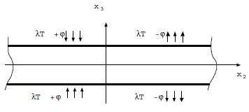
Figure: 3.2-a
The symmetry and antisymmetry conditions require the solution to verify:
\(-T({x}_{\mathrm{1,}}-{x}_{\mathrm{2,}}{x}_{3})=T({x}_{\mathrm{1,}}{x}_{\mathrm{2,}}{x}_{3})=T({x}_{\mathrm{1,}}{x}_{\mathrm{2,}}-{x}_{3})\)
from where: \(T({x}_{\mathrm{1,}}\mathrm{0,}{x}_{3})=0\), and \({\partial }_{3}T({x}_{\mathrm{1,}}{x}_{\mathrm{2,}}0)=0\).
The equations (18) can be written in our case (\({T}_{i}\) only depends on \({x}_{2}\)):
\(\{\begin{array}{ccc}-\text{kh}\text{.}{T}_{1}^{\text{'}\text{'}}+{\mathrm{\lambda T}}_{1}+{\mathrm{\lambda T}}_{3}& =\phi & \text{pour}{x}_{2}<0\text{ou}-\phi \text{pour}{x}_{2}>0\\ -\text{kh}/3\text{.}{T}_{2}^{\text{'}\text{'}}+(\frac{K}{h}+\lambda ){T}_{2}& =0& \\ -\text{kh}/5\text{.}{T}_{3}^{\text{'}\text{'}}+{\mathrm{\lambda T}}_{1}+(\frac{\mathrm{3K}}{h}+\lambda ){T}_{3}& =\phi & \text{pour}{x}_{2}<0\text{ou}-\phi \text{pour}{x}_{2}>0\end{array}\)
\({T}_{2}\) is therefore identically zero (which is consistent with the symmetry conditions).
Solutions \({\mathrm{T}}_{1}\) and \({\mathrm{T}}_{3}\) are given by (cf. [An 1]):
\(\{\begin{array}{}{T}_{1}({x}_{\mathrm{1,}}{x}_{2})=-\frac{\varphi }{\lambda }(1-\frac{\lambda /\mathrm{kh}-{s}_{2}^{2}}{{s}_{1}^{2}-{s}_{2}^{2}}\mathrm{.}{e}^{-{s}_{1}\mid {x}_{2}\mid }+\frac{\lambda /\mathrm{kh}-{s}_{1}^{2}}{{s}_{1}^{2}-{s}_{2}^{2}}\mathrm{.}{e}^{-{s}_{2}\mid {x}_{2}\mid })\mathrm{sgn}({x}_{2})\\ {T}_{3}({x}_{\mathrm{1,}}{x}_{2})=-\frac{\varphi }{\lambda }\mathrm{.}\frac{\mathrm{kh}}{\lambda }\frac{(\lambda /\mathrm{kh}-{s}_{2}^{2})\mathrm{.}(\lambda /\mathrm{kh}-{s}_{1}^{2})}{{s}_{1}^{2}-{s}_{2}^{2}}\mathrm{.}({e}^{-{s}_{1}\mid {x}_{2}\mid }-{e}^{-{s}_{2}\mid {x}_{2}\mid })\mathrm{sgn}({x}_{2})\end{array}\)
\({\mathrm{s}}_{1}\) and \({\mathrm{s}}_{2}\) being the positive roots of the characteristic polynomial.
After changing the variables \({T}^{m},{T}^{s},{T}^{i}\), we find:
\(\{\begin{array}{}{T}^{m}({x}_{\mathrm{1,}}{x}_{2})={T}_{1}({x}_{\mathrm{1,}}{x}_{2})\\ {T}^{s}({x}_{\mathrm{1,}}{x}_{2})={T}_{1}({x}_{\mathrm{1,}}{x}_{2})+{T}_{3}({x}_{\mathrm{1,}}{x}_{2})\\ {T}^{i}({x}_{\mathrm{1,}}{x}_{2})={T}^{s}({x}_{\mathrm{1,}}{x}_{2})\end{array}\)
If we adopt to solve the thermal problem a model with 2 fields \((\tilde{{T}_{\mathrm{1,}}}\tilde{{T}_{2}})\), with an affine representation in terms of thickness, we obtain as a solution:
\(\{\begin{array}{ccc}\tilde{{T}_{1}}({x}_{1},{x}_{2})=& \varphi /\lambda (1-{e}^{\sqrt{\lambda /\mathrm{kh}}\mathrm{.}{x}_{2}})& \text{si}({x}_{2}<0)\\ & -\varphi /\lambda (1-{e}^{\sqrt{\lambda /\mathrm{kh}}\mathrm{.}{x}_{2}})& \text{si}({x}_{2}>0)\\ \tilde{{T}_{2}}({x}_{1},{x}_{2})=& 0& \end{array}\)
In such a model, the temperature appears to be constant in the thickness. The asymptotic limit model produces the same solution.
We compare the 3D numerical solution and that of a model with 2 fields \((\tilde{{T}_{1}})\). This last comparison makes it possible to judge the effect of the parabolic term on the distribution of the mean temperature. In fact, it is the latter which, in the mechanical theory of shells, causes membrane deformation.
These comparisons are made for unit values of \(k,K,\lambda ,h,\varphi\) in Si units. We visualize the 3D isovalues in the thickness on the [Figure 3.3-a].
Average temperatures \({T}_{1}\) and \(\tilde{{T}_{1}}\) are shown [Figure 3.3-b]. Finally, the [Figure 3.3-c] shows the evolution of the temperature in the upper skin (\({x}_{3}=+h\)) of the plate, for the three solutions considered, as well as by that of the asymptotic limit model; the [Figure 3.3-d] presents the same comparison for the middle sheet of the plate.
These results show the good match between the complete 3D solution (points \(0\)) and that obtained with the shell model with 3 fields (points \(\Delta\)), while the model with 2 fields (points \(+\)) seems insufficient.
These observations remain valid for other choices of \(k,K,\lambda ,h,\varphi\), since the problem is linear in \(\varphi\), and the space variable \({x}_{2}\) appears to be normalized by \(\sqrt{\frac{\lambda }{\mathrm{kh}}}\) in the equations.

Figure: 3.3-a: Temperature isovalues by 3D numerical calculation
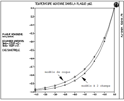
Figure: 3.3-b: Comparison of average temperatures: effect of the parabolic term
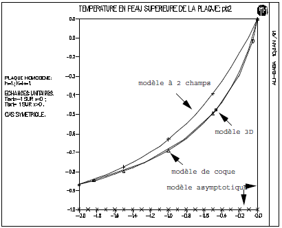
Figure: 3.3-c: Comparative temperature in the upper skin of the plate subject to symmetric exchanges
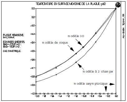
Figure: 3.3-d: Comparative temperature on the middle sheet of the plate subjected to symmetric exchanges
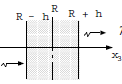
3.4. The infinite cylinder subjected to horizontal stratification#
This paragraph focuses on a situation that is more industrial than the previous cases. This is a thermal stratification problem in a horizontal pipe [bib12]. Under certain thermohydraulic conditions, the temperature of the fluid can vary very quickly with the \(z\) rating (see figure below). In practice, it can be considered that there are two zones with constant temperatures on either side of a horizontal interface.
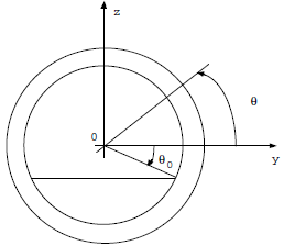
Figure: 3.4-a
Geometric characteristics:
\(R=\mathrm{1,0}m\) |
|
|
Physical characteristics:
Conductivity |
\(k=17W/m/°C\) |
Exchanges: |
outside (air) |
\(={\lambda }^{e}\) |
|
inside (hot water) |
\(={\lambda }^{c}\) |
|
|
inside (cold water) |
\(={\lambda }^{h}\) |
|
Determining the temperature in the pipe has two advantages, the first is to be able to lead to the distribution of stress in the vicinity of the stratification, the second is to estimate the heat exchanges between the « cold » water zone and the « hot » water zone via conduction in the tube.
Since the problem is independent of variable \(x\), it becomes one-dimensional as part of the shell model. To solve it, we first look for the general solutions of the equation without a second member on each of the segments \(\text{]}\mathrm{-}\frac{\pi }{2}\mathrm{,}{\theta }_{0}\text{[}\) and \(\text{]}{\theta }_{\mathrm{0,}}\frac{\pi }{2}\text{[}\):
\(-A\left[\begin{array}{}\Delta {T}_{1}\\ \Delta {T}_{2}\\ \Delta {T}_{3}\end{array}\right]+B\left[\begin{array}{}{T}_{1}\\ {T}_{2}\\ {T}_{3}\end{array}\right]=0\)
Solving a third-degree equation for this purpose numerically (characteristic polynomial \(s\)), the conditions of continuity of the \({T}_{i}\) fields and their tangential derivatives at the interface are then written, by expressing these by the combination of general solutions and particular solutions in each domain. The linear system to be solved (\(12\times 12\)) is brought back to a system of dimension \(6\times 6\) by symmetry considerations, then solved numerically.
We thus have a semi-analytical solution [bib4] (numerical resolution of the third-degree equation and the linear system) although the situation is complex. The comparison with a 2D finite element calculation is given on [Figure 3.4-b] and [Figure 3.4-c]: the difference between the two solutions is indistinguishable.
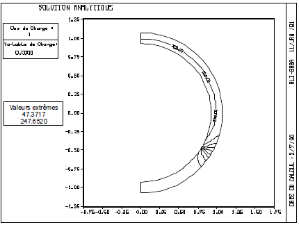
Figure 3.4-b: Stratified piping: analytical solution using the thermal shell model
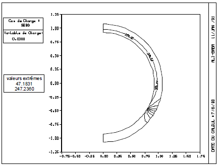
Figure 3.4-c: Stratified Piping: 2D Thermal Finite Element Solution Aster