4. Notes on digital discretization#
In this paragraph we are limited to a few observations concerning the numerical resolution of the equations of the thermal shell model: first of all on the use of a finite element method and then on the numerical block appearing when the thickness \(2h\) is low. The latter comes from the intervention of \(h\) at different powers in the coefficients of the equations.
4.1. Finite element resolution#
The shell thermal model described in [§ 2.3] has the following characteristics:
it leads to an operator of order \(2\) acting on the three scalar fields \(T=({T}^{m},{T}^{s},{T}^{i})\);
these three fields are defined on a \(\omega\) surface domain, immersed in \({ℝ}^{3}\);
the curvature of the surface \(\omega\) is, possibly, only involved in the expression of the coefficients \(A,B,C,D\).
In the general case of a shell of any shape immersed in \({ℝ}^{3}\), it is possible to discretize the geometry of its mean surface \(\omega\) by a mesh of plane triangular elements (this method certainly has the defect of not being able to explicitly take into account the curvature of \(\omega\)).
Since the thermal problem (see [§ 2.3.6]) is scalar, with \(3\) fields, of the second order, we propose the usual finite elements: the plane triangles \(\mathit{P1}\) (with \(3\) knots) or \(\mathit{P2}\) (with \(6\) knots).
Their formulation is the same, whether \(\omega\) is flat or curved: metric corrections are thus overlooked in stiffness operators \(A\) and \(B\) (we saw in validation cases that this had little effect in practice). On the other hand, if the user knows the curvature expression, it will be in his interest to take it into account in the values of the coefficients \({\lambda }^{\pm }\) and the flows \({\varphi }^{\pm }\), as in the expressions [éq2.3.1-4] and [éq 2.3.1-5].
In the case of composite materials (as well as if curvature was to be taken into account), it is necessary to provide a pre-treatment providing the coefficients \(A,B,C,D\), as well as a post-treatment to reconstitute the temperature and the flows at any point of the thickness.
There are situations where the problem only depends on a space variable: these are shells with axisymmetric load revolutions, or « shell slices », with axis \(\overrightarrow{{e}_{3}}\).
The geometry is then represented by a meridian: (see [Figure 4.1-a]). The average curve is then:
revolution case: \({H}_{1}=(\frac{1}{R}+\frac{\mathrm{cos}\alpha }{x})\)
« slice » case, or arc: \({H}_{1}=\frac{1}{R}\)
where \(R\) refers to the radius of curvature of the meridian line \(AB\).
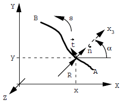
Figure 4.1-a.
For these types of problems, a finite element \(\mathit{P2}\) to \(3\) knots is also proposed, using the same formulation, where the metric correction in the thickness is neglected, for the coefficients \(A\) and \(B\). We use a 4-point quadrature formula from GAUSS.
This element is exactly associated with the one proposed in mechanics for chained thermo-mechanical studies [R3.07.02].
4.2. Numerical blocking of a finite thermal shell element#
Blocking is a phenomenon appearing in the numerical resolution by finite elements of certain problems such as that of thin shells or arcs when the element is curved (membrane blocking), that of shells or beams taking into account shear (shear blocking), or even that of plasticity (blocking of plastic incompressibility [bib7]). He was initially encountered in the mechanics of incompressible fluids and it was in this context that his theoretical study began [bib6].
This blocking phenomenon is manifested by a very great loss of precision and significant oscillations in certain quantities calculated when a physical parameter of the model becomes « small ». The illustration of these inconveniences is given in the note HI-71/7131, (§4.2). The origin of these problems lies in the order of magnitude difference that appears between certain components of the bilinear form of « stiffness » when the physical or geometric parameter tends to zero (shell thickness for membrane blocking, inverse of the tangent compressibility module for plastic blocking, for example). Here, it is the thickness of the shell that will play the role of small parameter.
Let’s go back to the equations of the stationary thermal problem posed on a plate in variational form; let’s note \(2\varepsilon h\) its thickness (\(\varepsilon\) real dimensionless):
\(\{\begin{array}{}\text{Trouver}T=({T}_{\mathrm{1,}}{T}_{\mathrm{2,}}{T}_{3})\in W(={\left[{H}_{0}^{1}(\omega )\right]}^{3})\text{tel que}\\ A(T,\theta )+\frac{1}{\varepsilon }B(T,\theta )=F(\theta )\text{}\forall \theta =({\theta }_{1},{\theta }_{\mathrm{2,}}{\theta }_{3})\in W\end{array}\) eq 4.2-1
with:
\(A(T,\theta )=\mathrm{2kh}{\int }_{\omega }[\nabla T]\mathrm{.}\left[\begin{array}{ccc}1& 0& 0\\ 0& \frac{1}{3}& 0\\ 0& 0& \frac{1}{5}\end{array}\right]\mathrm{.}[\nabla \theta ]d\omega\)
With \(\mathrm{.}\) designating the usual dot product,
\(B(T,\theta )=\frac{\mathrm{2K}}{h}{\int }_{\omega }[T]\mathrm{.}\left[\begin{array}{ccc}1& 0& 0\\ 0& 1& 0\\ 0& 0& 3\end{array}\right]\mathrm{.}[\theta ]d\omega\)
\([\nabla \theta ]=(\overrightarrow{\nabla }{\theta }_{1},\overrightarrow{\nabla }{\theta }_{2},\overrightarrow{\nabla }{\theta }_{3})\text{(gradients surfaciques)}\)
An equivalent mixed formulation of this problem is obtained with the variables \({\mathrm{q}}_{2}\) and \({\mathrm{q}}_{3}\), heat flow in the thickness (cf. [An 2]): we denote \(\theta ={({L}^{2}(\omega ))}^{2}\).
\(\{\begin{array}{}\text{Trouver}(T,[p])\in W\times Q\text{tels que}\\ \\ \{\begin{array}{}A(T,\theta )-M(\theta ,p)=F(\theta )\text{}\forall \theta \in W\\ -\varepsilon \stackrel{ˉ}{B}(p,q)-M(\theta ,q)=0\text{}\forall q\in Q\end{array}\end{array}\) eq 4.2-2
where:
\(\begin{array}{}[q]=({q}_{\mathrm{2,}}{q}_{3})\\ M(\theta ,q)={\int }_{\omega }({\theta }_{2}{q}_{2}+{\theta }_{3}{q}_{3})d\omega \\ \stackrel{ˉ}{B}(p,q)=\frac{h}{v}\mathrm{2K}{\int }_{\omega }[p]\left[\begin{array}{cc}1& 0\\ 0& \frac{1}{3}\end{array}\right][q]d\omega \end{array}\)
On this formulation, digital blocking is clear (at least formally). In fact, the discretization of \(W\times Q\) being carried out (it is noted \({W}_{d}\times {Q}_{d}\)), the problem formally tends when \(\varepsilon\) tends to zero to the following problem:
\(\{\begin{array}{cc}A({T}_{d},\theta )-M(\theta ,{p}_{d})& =F(\theta )\forall \theta \in {W}_{d}\\ M({T}_{d},q)& =0\text{}\forall q\in {Q}_{d}\end{array}\)
Which is the same as resolving on the \(M\) core:
\(A({T}_{d},\theta )=F(\theta )\forall \theta \in {W}_{d}\) eq 4.2-3
The blockage occurs when the discretized kernel of \(M\) is too small or reduced to zero: the resolution of [éq4.2-3] is done on a very small space or even reduced to zero. Even if the mesh is fine, the solution is then of very poor quality.
The core of \(M\) in \({W}_{d}\) being by definition, space:
\(\mathrm{Ker}{M}_{d}=\left\{\theta \in {W}_{d}\mid M(\theta ,q)=0\text{}\forall q\in {Q}_{d}\right\}\)
We can see that the choice to discretize \(Q\) is not an innocent step and strongly conditions the behavior of the solution when \(\varepsilon\) tends to zero. There is a convergence condition relating to the spaces \({W}_{d}\) and \({Q}_{d}\) which ensures the good numerical behavior of the solution with small, it is the so-called discrete LBB condition, a version adapted to the discrete case of the continuous LBB condition (LADYJENSKAIA - BREZZI - BABUCHKA). We refer to [bib 7] for a case study (plasticity) and a bibliography on this topic.
In parallel with the theoretical studies quickly mentioned above, a practical remedy for blocking, appearing once the discretization in \({W}_{d}\) has been chosen if this choice has been unfortunate, consists in under-integrating the term « blocker » into the construction of rigidity, i.e. the B term here. Some sub-integration choices, in the primal formulation [éq 4.2-1], are interpreted as interpolation choices of \({W}_{d}\) and \({Q}_{d}\) in the mixed formulation and can thus, via the (sometimes painstaking) verification of the discrete LBB condition, be justified theoretically.
Indeed, consider a triangular finite element with 3 nodes and interpolation \(\mathit{P1}\) to solve the problem [éq 4.2-2]. Let us then choose to discretize \(Q\) a discontinuous \(\mathit{P0}\) interpolation, that is to say a representation of \(\mathrm{[}q\mathrm{]}\) constant by element.
The second equation of [éq 4.2-2] is then a local equation, that is to say to be solved on each element separately since \(p\) is arbitrary on each element \(E\).
\(-\frac{\varepsilon h}{\mathrm{2K}}{\int }_{E}({p}_{2}{q}_{2}+\frac{1}{3}{p}_{3}{q}_{3})-{\int }_{E}{T}_{2}{q}_{2}+{T}_{3}{Q}_{3}=0\text{}\forall ({q}_{\mathrm{2,}}{q}_{3})\)
Hence the immediate solution if \(\mid E\mid\) is the surface of \(E\).
\(\{\begin{array}{}{p}_{2}=-\frac{\mathrm{2K}}{\varepsilon h}\frac{1}{\mid E\mid }{\int }_{E}{T}_{2}\\ {p}_{3}=-\frac{\mathrm{6K}}{\varepsilon h}\frac{1}{\mid E\mid }{\int }_{E}{T}_{3}\end{array}\)
By reporting these results in the form \(M\), we have on the element \(E\):
\(\mathrm{M}(\theta \mathrm{,}\mathrm{p})\mathrm{=}\frac{\mathrm{2K}}{\varepsilon \mathrm{h}}\left[\frac{1}{\mathrm{\mid }\mathrm{E}\mathrm{\mid }}{\mathrm{\int }}_{\mathrm{E}}{\mathrm{T}}_{2}{\mathrm{\int }}_{\mathrm{E}}{\theta }_{2}+\frac{3}{\mathrm{\mid }\mathrm{E}\mathrm{\mid }}{\mathrm{\int }}_{\mathrm{E}}{\mathrm{T}}_{3}{\mathrm{\int }}_{\mathrm{E}}{\theta }_{3}\right]\) for everything \(\theta \mathrm{\in }{W}_{d}\)
having thus eliminated \(p\), we are brought back to a primal formulation on \(T\) only:
\(M(\theta ,p)=\frac{\mathrm{2K}}{\varepsilon h}\left[\frac{1}{\mid E\mid }{\int }_{E}{T}_{2}{\int }_{E}{\theta }_{2}+\frac{3}{\mid E\mid }{\int }_{E}{T}_{3}{\int }_{E}{\theta }_{3}\right]\text{pour tout}\theta \in {W}_{d}\)
which corresponds very exactly to the formulation [éq 4.2-1] in which the elementary term:
\({B}_{E}(T,\theta )=\frac{\mathrm{2K}}{\varepsilon h}{\int }_{E}({T}_{2}{\theta }_{2}+3{T}_{3}{\theta }_{3})\)
is under-integrated by a schema at a point of GAUSS:
\({\int }_{E}\mathrm{f.g}=\frac{1}{\mid E\mid }\mathrm{.}{\int }_{E}f\mathrm{.}{\int }_{E}g\mathrm{.}\)
The examination of the discrete LBB condition remains to be done for this discretization in order to conclude that it has converged (cf. [bib7]).