7. Description of document versions

Version Aster	Author (s) Organization (s)	Description of changes
2.6	F. VOLDOIRE, S. ANDRIEUX (EDF/IMA/MMN)	Initial text
11.3	F. VOLDOIRE, (EDF/AMA)	Typing corrections (rex sheet 20336) and addition of figures from the initial version.

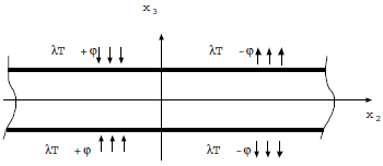
Infinite plate under a couple of symmetric flows

In \({x}_{3}=+h\), the boundary conditions are:

\(\begin{array}{cc}-K{\partial }_{3}T& =\lambda T+\varphi \text{si}{x}_{2}<0\\ & =\lambda T-\varphi \text{si}{x}_{2}>0\end{array}\)

In \({x}_{3}=-h\), we have:

\(\begin{array}{cc}-K{\partial }_{3}T& =-\lambda T+\varphi \text{si}{x}_{2}<0\\ & =-\lambda T-\varphi \text{si}{x}_{2}>0\end{array}\)

\({T}_{i}(\mathrm{0,}0)=0\)

The symmetry and antisymmetry conditions require the solution to verify:

\(-T({x}_{\mathrm{1,}}-{x}_{\mathrm{2,}}{x}_{3})=T({x}_{\mathrm{1,}}{x}_{\mathrm{2,}}{x}_{3})=T({x}_{\mathrm{1,}}{x}_{\mathrm{2,}}-{x}_{3})\)

and so: \(T({x}_{\mathrm{1,}}\mathrm{0,}{x}_{3})=0\), \({\partial }_{3}T({x}_{\mathrm{1,}}{x}_{\mathrm{2,}}0)=0\).

The equations [éq 2.3.2-2] are written in our case:

\(\{\begin{array}{ccc}-\text{kh}\text{.}{T}_{1}^{\text{'}\text{'}}+{\mathrm{\lambda T}}_{1}+{\mathrm{\lambda T}}_{3}& =\phi & \text{pour}{x}_{2}<0\text{ou}-\phi \text{pour}{x}_{2}>0\\ -\text{kh}/3\text{.}{T}_{2}^{\text{'}\text{'}}+(\frac{K}{h}+\lambda ){T}_{2}& =0& \\ -\text{kh}/5\text{.}{T}_{3}^{\text{'}\text{'}}+{\mathrm{\lambda T}}_{1}+(\frac{\mathrm{3K}}{h}+\lambda ){T}_{3}& =\phi & \text{pour}{x}_{2}<0\text{ou}-\phi \text{pour}{x}_{2}>0\end{array}\)

\({T}_{2}\) is therefore identically zero (which is consistent with the symmetry conditions). The previous system admits as a particular solution:

\(\{\begin{array}{}{T}_{1}^{p}({x}_{1},{x}_{2})=\frac{j}{\lambda }\text{si}{x}_{2}<0\text{et}-\frac{j}{\lambda }\text{si}{x}_{2}>0\\ {T}_{3}^{p}({x}_{1},{x}_{2})=0\mathrm{sur}{R}^{2}\end{array}\)

The characteristic polynomial in s of the homogeneous system is:

\(\frac{{k}^{2}{h}^{2}}{5}{s}^{4}-k(\frac{6h\lambda }{5}+3K){s}^{2}+\frac{3\lambda K}{h}=0\), whose 4 \({s}_{i}\) roots are:

\({s}_{i}=\pm \frac{1}{h}\mathrm{.}\sqrt{\frac{3}{k}}\mathrm{.}\sqrt{(\lambda h+\frac{5}{2}K)\pm \sqrt{{\lambda }^{2}{h}^{2}+\frac{25{K}^{2}}{4}+\frac{10K\lambda h}{3}}}\text{,}{s}_{1}>{s}_{2}>0>{s}_{3}>{s}_{4}\)

The solutions \({T}_{1}({x}_{1},{x}_{2})\) and \({T}_{3}({x}_{1},{x}_{2})\), finished in \(\mid {x}_{2}\mid =\infty\), are therefore expressed:

\(\begin{array}{ccc}{T}_{1}({x}_{1},{x}_{2})& =\frac{\varphi }{\lambda }+\alpha {e}^{{s}_{1}{x}_{2}}+\beta {e}^{{s}_{2}{x}_{2}}& \text{pour}{x}_{2}>0\\ & =-\frac{\varphi }{\lambda }-\alpha {e}^{-{s}_{1}{x}_{2}}-\beta {e}^{-{s}_{2}{x}_{2}}& \text{pour}{x}_{2}>0\\ {T}_{3}({x}_{1},{x}_{2})& =\gamma {e}^{{s}_{1}{x}_{2}}+\delta {e}^{{s}_{2}{x}_{2}}& \text{pour}{x}_{2}>0\\ & =-\gamma {e}^{-{s}_{1}{x}_{2}}-\delta {e}^{-{s}_{2}{x}_{2}}& \text{pour}{x}_{2}>0\end{array}\)

The connection conditions in \({x}_{2}=0\) are naturally expressed by the antisymmetry conditions in \(T\), already used above. The four constants \(\alpha ,\beta ,\gamma ,\delta\) are determined by:

\(\{\begin{array}{}\begin{array}{}\alpha +\beta =-\varphi /\lambda \\ \gamma +\delta =0\end{array}\}\mathrm{nullité}\mathrm{de}T\mathrm{en}{x}_{2}=0\\ \begin{array}{}\alpha (\lambda -\mathrm{kh}{s}_{1}^{2})+\gamma \lambda =0\\ \beta (\lambda -\mathrm{kh}{s}_{2}^{2})+\delta \lambda =0\end{array}\}\mathrm{modes}{T}_{1}-{T}_{3}\mathrm{associés}à{s}_{1},{s}_{2}\end{array}\)

From where:

\(\{\begin{array}{}\alpha =-\frac{\varphi }{\lambda }\mathrm{.}\frac{(\lambda /\mathrm{kh}-{s}_{2}^{2})}{{s}_{1}^{2}-{s}_{2}^{2}}\\ \beta =\frac{\varphi }{\lambda }\mathrm{.}\frac{(\lambda /\mathrm{kh}-{s}_{1}^{2})}{{s}_{1}^{2}-{s}_{2}^{2}}\\ \gamma =\frac{\varphi \mathrm{.}\mathrm{kh}}{{\lambda }^{2}}\mathrm{.}\frac{(\lambda /\mathrm{kh}-{s}_{2}^{2})\mathrm{.}(\lambda /\mathrm{kh}-{s}_{1}^{2})}{{s}_{1}^{2}-{s}_{2}^{2}}\\ \delta =\frac{\varphi \mathrm{.}\mathrm{kh}}{{\lambda }^{2}}\mathrm{.}\frac{(\lambda /\mathrm{kh}-{s}_{2}^{2})\mathrm{.}(\lambda /\mathrm{kh}-{s}_{1}^{2})}{{s}_{1}^{2}-{s}_{2}^{2}}\end{array}\)

So solutions \({\mathrm{T}}_{1}\) and \({\mathrm{T}}_{3}\) are written as:

\(\{\begin{array}{}{T}_{1}({x}_{1},{x}_{2})=-\frac{\varphi }{\lambda }\mathrm{.}(1-\frac{\lambda /\mathrm{kh}-{s}_{2}^{2}}{{s}_{1}^{2}-{s}_{2}^{2}}{e}^{-{s}_{1}\mid {x}_{2}\mid }+\frac{\lambda /\mathrm{kh}-{s}_{1}^{2}}{{s}_{1}^{2}-{s}_{2}^{2}}{e}^{-{s}_{2}\mid {x}_{2}\mid })\mathrm{sgn}({x}_{2})\\ {T}_{3}({x}_{1},{x}_{2})=-\frac{\varphi \mathrm{.}\mathrm{kh}}{{\lambda }^{2}}\mathrm{.}\frac{(\lambda /\mathrm{kh}-{s}_{2}^{2})\mathrm{.}(\lambda /\mathrm{kh}-{s}_{1}^{2})}{{s}_{1}^{2}-{s}_{2}^{2}}\mathrm{.}({e}^{-{s}_{1}\mid {x}_{2}\mid }-{e}^{-{s}_{2}\mid {x}_{2}\mid })\mathrm{sgn}({x}_{2})\end{array}\)

Mixed formulation of the stationary problem for plaque

In the case of the plate, the variational problem [éq 4.2-1] is equivalent to a minimization problem (by making the thickness \(\varepsilon h\) appear explicitly in \(B\)) of the functional:

\(J(\theta )=\frac{1}{2}A(\theta ,\theta )+\frac{1}{2\varepsilon }B(\theta ,\theta )-F(\theta )\)

To obtain the mixed formulation, note that:

Proposal:

\(\frac{1}{2\varepsilon }B(\theta ,\theta )=\underset{({q}_{\mathrm{2,}}{q}_{3})\in {\left[{L}^{2}(\omega )\right]}^{2}}{\text{Sup}}\left[-{\int }_{\omega }({q}_{2}{\theta }_{2}+{q}_{3}{\theta }_{3})-\frac{\varepsilon }{4}\frac{h}{K}{\int }_{\omega }({q}_{1}^{2}+\frac{1}{3}{q}_{3}^{2})\right]\)

Demonstration:

Let’s write the extremality condition of the functional in square brackets (its opposite is strictly convex, coercive and semi-continuous at the bottom) and let p denote the couple where the sup is reached:

\({q}_{2}{\theta }_{2}+{q}_{3}{\theta }_{3}+\frac{\varepsilon }{2}\frac{h}{K}({q}_{2}{p}_{2}+\frac{1}{3}{q}_{3}{p}_{3})=0\text{}\forall q\)

from where: \(\{\begin{array}{}{p}_{2}=-\frac{2K}{\varepsilon h}{\theta }_{2}\\ {p}_{3}=-\frac{6K}{\varepsilon h}{\theta }_{3}\end{array}\)

The value of the functional at this point is therefore:

\({\int }_{\omega }+\frac{\mathrm{2K}}{\varepsilon h}{\theta }_{2}^{2}+\frac{\mathrm{6K}}{\varepsilon h}{\theta }_{3}^{2}-\frac{\varepsilon h}{4K}\left[\frac{4{K}^{2}}{{\varepsilon }^{2}{h}^{2}}{\theta }_{2}^{2}+\frac{{\mathrm{36K}}^{2}}{3{\varepsilon }^{2}{h}^{2}}{\theta }_{3}^{2}\right]=\frac{1}{\varepsilon h}\left[\frac{\mathrm{2K}}{h}{\theta }_{2}^{2}+\frac{\mathrm{3K}}{h}{\theta }_{3}^{2}\right]\)

is in fact the announced result.

So we have a formulation equivalent to the minimization of \(J\) over \(W\):

\(\underset{\theta \mathrm{\in }\mathrm{W}}{\mathrm{Min}}\underset{\mathrm{q}\mathrm{\in }\mathrm{Q}}{\mathrm{Max}}\left[\frac{1}{2}\mathrm{A}(\theta \mathrm{,}\theta )\mathrm{-}\frac{\varepsilon }{2}\stackrel{ˉ}{\mathrm{B}}(\mathrm{q}\mathrm{,}\mathrm{q})\mathrm{-}\mathrm{M}(\theta \mathrm{,}\mathrm{q})\mathrm{-}\mathrm{F}(\theta )\mathrm{.}\right]\)

by noting:

\(M(\theta ,q)={\int }_{\omega }{q}_{2}{\theta }_{2}+{q}_{3}{\theta }_{3}\text{,}\stackrel{ˉ}{B}(q,q)={\int }_{\omega }\frac{h}{\mathrm{2K}}({p}_{2}{q}_{2}+\frac{1}{3}{p}_{3}{q}_{3})\)

The saddle point condition of this Lagrangian leads to the formulation [éq 4.2 - 2]:

\(\{\begin{array}{}A(T,\theta )-M(\theta ,p)=F(\theta )\text{}\forall \theta \in W\\ -\varepsilon \stackrel{ˉ}{B}(p,q)-M(T,q)=0\text{}\forall q\in Q\end{array}\)