2. Presentation of the model#
2.1. Position of the thermal problem in shells#
In this paragraph, we will first recall the description of the geometry of shells, seen as thin three-dimensional solids. The thermal conduction problem will then be posed.
2.1.1. Geometry description#
A shell is defined as being a solid \(\Omega\), thin perpendicular to an average surface \(\omega\). Note the thickness of the shell \(\mathrm{2h}\); we choose a coordinate system \(({x}_{\mathrm{1,}}{x}_{2})\) on the surface \(\omega\). We note \(g\) the associated metric tensor, \(\overrightarrow{n}\) the normal vector, the normal vector, \(c\) the curvature of \(\omega\) tensor.
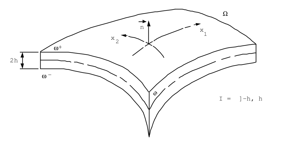
Figure: 2.1.1-a
Shell \(\Omega\) is described by the coordinate system \(({x}_{\gamma },{x}_{3})\), \({x}_{3}\) according to \(\overrightarrow{n}\): \(\Omega =\omega \times \text{] - h, h[}\)
(Greek indices \(\alpha ,\beta ,\gamma\) are dedicated to surface coordinates on \(\omega\)).
This description is of course suitable for a shell whose thickness \(\mathrm{2h}\) is less than the smallest radius of curvature of \(\omega\).
At any point \(({x}_{\gamma },{x}_{3})\) in shell \(\Omega\), the metric tensor \(G\) is expressed as a function of the fundamental tensors \(g\) and \(c\) of the mean surface \(\omega\) by:
\(\{\begin{array}{}{G}_{\alpha \beta }({x}_{\gamma },{x}_{3})={g}_{\alpha ,\beta }({x}_{\gamma })-2{x}_{3}{c}_{\alpha \beta }({X}_{\gamma })\\ {G}_{\alpha 3}=0\text{},\text{}{G}_{33}=1\end{array}\) eq 2.1.1-1
and \(\begin{array}{cc}\sqrt{\text{det}G}& \text{=}\sqrt{\text{det}G}(1-{x}_{3}\text{tr}c)\\ & \text{=}\sqrt{\text{det}G}(1+{x}_{3}(\frac{1}{{R}_{1}}+\frac{1}{{R}_{2}}))\end{array}\)
where \({R}_{\mathrm{1,}}{R}_{2}\) are the main radii of curvature of \(\omega\) at the point \({x}_{\gamma }\) under consideration.
Note:
We actually know that the trace \((\mathrm{tr})\) of a tensor is an invariant (by base change). However, we are used to writing quantities on a physical basis, that is to say orthonormal. So: . \({G}_{\alpha \beta }^{\text{phy}}({x}_{\gamma },{x}_{3})={\delta }_{\alpha \beta }-2{x}_{3}{C}_{\alpha \beta }^{\text{phy}}({x}_{\gamma })\)
And if the base is the main curvature: \({C}_{\alpha \beta }^{\text{phy}}=\frac{-1}{{R}_{\beta }}{\delta }_{\alpha \beta }\) (without summation) .
Note: \(\frac{1}{{R}_{1}}+\frac{1}{{R}_{2}}={H}_{1}\) and \(\frac{1}{{R}_{1}}-\frac{1}{{R}_{2}}={H}_{2}\).
We have limited ourselves here to the terms of the first order in \({x}_{3}\text{tr}C\); as we will do throughout the rest of the following. In practice, in fact, the thinness of the shell allows such simplification. It will also be advantageous to place ourselves in a main coordinate system of curvature, orthonormal. The tensor \(g\) is then the identity, \(C\) is diagonal. That’s what we’re going to do from now on.
2.1.2. Heat equation#
The equations of three-dimensional heat conduction are written (for a rigid conductor):
\(-\text{div}(K\overrightarrow{\mathrm{grad}}T)+\rho {C}_{t}T=r\) eq 2.1.2-1
where \(K\) designates the conductivity tensor, \(\rho C\) the calorific capacity and \(r\) the possible sources.
It is advantageous to write the expression for the differential operator according to the metric \(G\) generated by the mean area \(\omega\). In fact, isotropic conductivity tensors \(K\) that are transverse along these coordinate axes will in fact be considered (cf. multilayer materials).
\({K}_{j}^{i}=(\begin{array}{cc}{k}_{\beta }^{\alpha }& 0\\ 0& K\end{array}),{k}_{\beta }^{\alpha }\mathrm{et}K\mathrm{pouvant}\mathrm{varier}\mathrm{avec}{x}_{\mathrm{1,}}{x}_{\mathrm{2,}}{x}_{3}\)
The operator expression:
\(-\text{div}(K\overrightarrow{\mathrm{grad}}T)=-{(\text{det}G)}^{-1/2}\mathrm{.}{\partial }_{i}(\text{det}{G}^{1/2}{K}_{j}^{i}{G}^{ij}{\partial }_{j}T)\)
is then written in the first order in \({x}_{3}/\text{tr}c\), for orthotropic conductivity according to the main directions of curvature:
\(-(1-{x}_{3}{H}_{1})\mathrm{.}\left[{\partial }_{1}\left[(1-{x}_{3}{H}_{2}){k}_{11}{\partial }_{1}T\right]+{\partial }_{2}\left[(1+{x}_{3}{H}_{2}){k}_{22}{\partial }_{2}T\right]+{H}_{1}K{\partial }_{3}T\right]-{\partial }_{3}\left[K{\partial }_{3}T\right]\) eq 2.1.2-2
If the curvatures are constant, this becomes:
\(-(1-2{x}_{3}/{R}_{1})\mathrm{.}({\partial }_{1}({k}_{11}{\partial }_{1}T))-(1-2{x}_{3}/{R}_{2})\mathrm{.}({\partial }_{2}({k}_{22}{\partial }_{2}T))-{H}_{1}(1-{x}_{3}{H}_{1})K{\partial }_{3}T-{\partial }_{3}(K{\partial }_{3}T)\)
The effect of curvature is therefore of the same type as a modified distribution of conductivity in thickness.
2.1.3. Thermal for a thin structure#
The equations of stationary heat on the shell can be written in the form of a minimization problem.
In particular, it is assumed that the boundary conditions on the ends \(\partial \omega \times I\) of the shell \(\Omega\) are of the same type over the entire thickness \(I\). We partition \(\partial \omega \times I\) into:
\(\partial {\omega }_{T}\times I\) (zone with imposed temperature),
and \(\partial {\omega }_{\varphi }\times I\) (zone subject to exchange or imposed flow).
\(\{\begin{array}{}\mathrm{Trouver}\text{le}\mathrm{champ}\mathrm{de}\mathrm{température}T:\\ \\ T=\underset{\theta \in V}{\mathrm{Arg}}\mathrm{Min}J(\theta ),\mathrm{avec}J(\theta )=\frac{1}{2}A(\theta ,\theta )-F(\theta ),\mathrm{avec}:\\ \\ A(T,\theta )={\int }_{\Omega }\mathrm{K.}\Delta \mathrm{T.}\Delta \theta d\Omega +{\int }_{{\omega }^{+}\cup {\omega }^{-}}\lambda T\mathrm{.}\theta d{\omega }^{\pm }+{\int }_{\partial {\omega }_{\varphi }\times I}\lambda \mathrm{T.}\theta dS\\ \\ F(\theta )={\int }_{{\omega }^{+}\cup {\omega }^{-}}\varphi \mathrm{.}\theta d{\omega }^{\pm }+{\int }_{\partial {\omega }_{\varphi }\times I}\varphi \mathrm{.}\theta dS\end{array}\) eq 2.1.3-1
We note:
\(V=\left\{\theta \in {H}^{1}(\omega \times I),\theta =0\mathrm{sur}\partial {\omega }_{T}\times I\right\}\).
The boundary conditions on \({\omega }^{+}\cup {\omega }^{-}\cup (\partial {\omega }_{\varphi }\times I)\) are of the type exchange or imposed flow \(\varphi\):
\(\overrightarrow{\Phi }\overrightarrow{n}=\lambda T-\varphi =-(K\Delta T)\mathrm{.}\overrightarrow{n}\) \(\lambda\) being an exchange coefficient.
The conductivity term in \(A(T,\theta )\) is written as:
\({\int }_{\Omega }K\Delta \mathrm{T.}\Delta \theta d\Omega\)
\(={\int }_{\omega }{\int }_{I}\left[{k}_{\alpha \beta }(1-{x}_{3}(\frac{1}{{R}_{\alpha }}+\frac{1}{{R}_{\beta }})){\partial }_{\alpha }T{\partial }_{\beta }\theta +K{\partial }_{3}T{\partial }_{3}\theta \right](1+{x}_{3}{H}_{1}){\mathrm{dx}}_{1}{\mathrm{dx}}_{2}{\mathrm{dx}}_{3}\)
This, in an orthonormal main coordinate system with a curvature of \(\omega\) (\({k}_{\alpha \beta }\) and \(K\) are then the physical components of the conduction tensor \(K\)).
The terms of trade on surfaces \({\omega }^{+}\) and \({\omega }^{-}\) are:
\({\int }_{{\omega }^{+}\cup {\omega }^{-}}\varphi \mathrm{.}\theta d{\omega }^{\pm }={\int }_{\omega }{\lambda }^{\pm }{T}^{\pm }{\theta }^{\pm }\mathrm{.}(1\pm h\mathrm{.}{H}_{1}){\mathrm{dx}}_{1}{\mathrm{dx}}_{2}\)
The object of a thermal shell model is therefore to reduce the dependence of the temperature field \(T\) in the expression of the differential operator corresponding to [eq 2.1.2-2] or [eq 2.1.3-1] from three to two space variables, by choosing and justifying appropriate hypotheses.
The model proposed in [§2.3] is based on the results of the asymptotic development of the thermal equations presented in [§2.2] below.
2.2. Summary of the results of asymptotic development#
2.2.1. The limit model obtained#
Here we summarize the main results obtained in [bib1] by an asymptotic development technique. We consider the case of a plate: \(\omega \times {I}_{\varepsilon }\), \(2\varepsilon h\) thick. The temperature is set to \(0\) on edge \(\partial \omega \times {I}_{\varepsilon }\), and flows \({\varphi }^{+}\), \({\varphi }^{-}\) on faces \({\omega }^{+}\) and \({\omega }^{-}\).
The aim is to study the dependence of solution \({T}^{\varepsilon }\) of the thermal problem [éq 2.1.3-1] on the thickness of the plate \(2\varepsilon h\). To do this, we use an open change technique that brings the problem back to a fixed domain \(\omega \times I\), with \(i=\text{]}-h,+h\text{[}\). The parameter \(\varepsilon\) then appears explicitly in the equations of the transported problem \(({P}^{\varepsilon })\), from \(\omega \times {I}_{\varepsilon }\) to \(\omega \times I\).
On \(\omega \times {I}_{\varepsilon }\), the initial problem is written in variational form:
\(\{\begin{array}{}\mathrm{Trouver}:{T}^{\varepsilon }\in V=\text{{}\theta \in {H}^{1}(\omega \times {I}_{\varepsilon }),\theta =0\mathrm{sur}\partial \omega \times {I}_{\varepsilon }\text{}}\\ \mathrm{tel}\mathrm{que}:\\ {\int }_{\omega \times {I}_{\varepsilon }}({k}_{\alpha \text{}\mathrm{bêta}}\mathrm{.}{T}_{,\alpha }\mathrm{.}{\theta }_{,\beta }+{k}_{\text{33}}{T}_{\text{'}3}\mathrm{.}{\theta }_{\text{'}3})={\int }_{\omega }({\varphi }^{+}{\theta }^{+}+\varphi -{\theta }^{-})\text{}\forall \theta \text{}{V}^{\varepsilon }\end{array}\) eq 2.2.1-1
The results of the asymptotic development [bib 1] consist of the following properties verified by \(T(\varepsilon )\), the solution of the transported problem \(({\mathrm{P}}^{\varepsilon })\), posed on \(\omega \times I\):
\(\{\begin{array}{cc}(i)& \frac{1}{\varepsilon }T(\varepsilon )\mathrm{tend}\mathrm{vers}{T}_{1}({x}_{\alpha };{x}_{3})={T}_{1}({x}_{\alpha })\mathrm{dans}{H}^{1}(\omega \times I)\\ & {T}_{1}({x}_{\alpha })\mathrm{apparaît}\mathrm{comme}\mathrm{une}\mathrm{température}\mathrm{moyenne}\mathrm{sur}l\text{'}\mathrm{épaisseur}I,\mathrm{au}\mathrm{point}{x}_{\alpha }\\ (\mathrm{ii})& \varepsilon T,∍(\varepsilon ),\mathrm{qui}\mathrm{est}\mathrm{la}\mathrm{dérivée}\mathrm{de}\varepsilon T\mathrm{selon}\mathrm{la}\mathrm{variable}d\text{'}\mathrm{épaisseur}{x}_{3}\in I,\mathrm{tend}\mathrm{vers}\mathrm{la}\mathrm{dérivée}\mathrm{selon}{x}_{3}\\ & \mathrm{du}\mathrm{champ}\rho ({x}_{\alpha };{x}_{3})\mathrm{dans}{L}^{2}(\omega )\times {H}_{m}^{1}(I),\mathrm{où}{H}_{m}^{1}(I)\mathrm{désigne}l\text{'}\mathrm{espace}\mathrm{des}\mathrm{fonctions}\mathrm{de}\\ & {H}^{1}(I)à\mathrm{moyenne}\mathrm{nulle.}\end{array}\) eq 2.2.1-2
In conclusion, the solution \({T}^{\varepsilon }\) of the initial problem on \(\omega \times {I}_{\varepsilon }\) can be represented by the first two terms of its development:
\({T}^{\varepsilon }({x}_{\alpha },{x}_{∍}^{\varepsilon })=\frac{1}{\varepsilon }{T}_{1}({x}_{\alpha })+\varepsilon \rho ({x}_{\alpha },{x}_{3}={x}_{∍}^{\varepsilon }/\varepsilon )+\mathrm{....}\) eq 2.2.1-3
However, the \({T}^{\varepsilon }\) gradient is not represented by the \({T}^{\varepsilon }\) representation gradient. This situation is generic for the problems of singular disturbances encountered in the study of thin structures (plates, beams, etc.). ):
\({(\nabla {T}^{\varepsilon })}^{\varepsilon }({x}_{\alpha },{x}_{∍}^{\varepsilon })=\frac{1}{\varepsilon }{T}_{1}{({x}_{\alpha })}_{\text{'}\beta }\overrightarrow{{e}_{\beta }}+\rho {({x}_{\alpha },{x}_{3}={x}_{∍}^{\varepsilon }/\varepsilon )}_{\text{'}∍}\overrightarrow{{e}_{3}}\) eq 2.2.1-4
So the « \({T}^{\varepsilon }\) gradient » field is not a gradient field!
Fields \({T}_{1}\) and \(\rho\) are calculated on the average area \(\omega\). In the case where the conductivity is homogeneous in thickness, we have:
\(\{\begin{array}{}{T}_{1}\in {H}_{0}^{1}(\omega ),\mathrm{solution}\mathrm{de}:\\ {\int }_{\omega }h{k}_{\alpha \beta }{T}_{\mathrm{1,}\alpha }\mathrm{.}{\theta }_{\text{'}\beta }={\int }_{\omega }\frac{1}{2}({\varphi }^{+}+{\varphi }^{-})\theta ,\text{}\forall \theta \in {H}_{0}^{1}(\omega )\end{array}\) eq 2.2.1-5
\(\rho ({x}_{\alpha },{x}_{3})=\frac{{\varphi }^{+}({x}_{\alpha })+{\varphi }^{-}({x}_{\alpha })}{4K({x}_{\alpha })}\mathrm{.}(\frac{{x}_{3}^{2}}{h}-\frac{h}{3})+\frac{{\varphi }^{+}({x}_{\alpha })-{\varphi }^{-}({x}_{\alpha })}{2K({x}_{\alpha })}\mathrm{.}{x}_{3}\) eq 2.2.1-6
We note that \({T}_{1}\) is the solution of a problem posed on \(\omega\), while \(\rho\) is obtained explicitly according to the flows imposed. These two equations constitute the « limit » model obtained by the asymptotic expansion.
Note:
In a more graphic and fuzzy language, the previous results are interpreted by saying that for a thin plate, the average temperature is governed by the average flow received and the conduction in the plane of the plate. The distribution in thickness is a function, at a given point, only of the flows imposed at this point on the upper and lower faces; it is not affected by the presence of neighboring points.
The temperature distribution in the thickness is « parabolic » according to the representation [éq 2.2.1-6].
2.2.2. An application#
The results of asymptotic development can be illustrated by a simple example, which also shows the limitations of the model obtained by using the temperature representation [éq2.2.1-3] using the \({T}_{1}\) and \(\rho\) fields, [éq 2.2.1-5] and [éq 2.2.1-6] fields.
We consider an infinite plate subjected on its \({x}_{2}<0\) half to a pair of balanced \(({\varphi }^{+}=\varphi ,{\varphi }^{-}=-\varphi )\) constant flows, and isolated on the other half \({x}_{2}>0\).

Figure: 2.2.2-a
The problem [eq 2.2.1-5] of determining the mean temperature \({T}_{1}\) is here a differential equation in \({x}_{2}\): \(\frac{{\partial }^{2}{x}_{2}}{\partial {x}_{2}^{2}}{T}_{1}({x}_{2})=0\) since the average flow \({j}^{+}+{j}^{-}\) is zero. The solution is then \({T}_{1}=0\) everywhere.
Field \(\rho ({x}_{\mathrm{2,}}{x}_{3})\) is easily calculated by [éq 2.2.1-6] :`
\(\rho ({x}_{\mathrm{2,}}{x}_{3})=\frac{\varphi }{K}\mathrm{.}{x}_{3}\) |
for \({x}_{2}<0\), |
\(\rho ({x}_{\mathrm{2,}}{x}_{3})=0\) |
for \({x}_{2}>0\). |
The discontinuity of the condition at the limits of NEUMANN on \({\omega }^{\pm }\) therefore relates directly to the temperature field: on the upper side the temperature \(T\) is as follows:
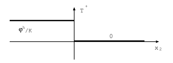
Figure: 2.2.2-b
This discontinuity also appears to be independent of the thickness \(h\) in this limit model, once the flow \(\varphi\) provided has been normalized by \(h\).
This limitation of the limit model obtained by asymptotic development is inherent in the purely local determination of the complementary parabolic term \(\rho ({x}_{\alpha },{x}_{3})\). The induced discontinuities will be annoying for applications, especially in thermomechanics.
It is thus necessary to formulate the shell thermal model differently, while maintaining the results of this asymptotic development.
2.3. Formulation of the stationary thermal shell model#
We saw from the results of the asymptotic study of the three-dimensional equations on solid \(\Omega =\omega \times I\), that the limit model obtained included an average temperature solution of a 2nd order problem posed on \(\omega\), and that the additional parabolic term was determined only locally (point by point on \(\omega\)). This therefore had the disadvantage of providing discontinuous solutions when the thermal « loads » are discontinuous.
In this paragraph, we therefore present a representation of the temperature, which is always parabolic in terms of thickness, but avoiding the previous pitfall. The equations obtained and their properties are described.
2.3.1. Model equations#
Following the results of the asymptotic development, we choose the representation in the following thickness on \(\Omega =\omega \times I\):
\(T({x}_{\alpha },{x}_{3})={T}_{1}({x}_{\alpha })+{T}_{2}({x}_{\alpha })\mathrm{.}{w}_{2}({x}_{3})+{T}_{3}({x}_{\alpha })\mathrm{.}{w}_{3}({x}_{3})\) eq 2.3.1-1
with \(({w}_{1}=\mathrm{1,}{w}_{\mathrm{2,}}{w}_{3})\) a database of degree 2 polynomials.
The determination of the field \(T\) with three space variables is thus replaced by that of three scalar fields \({T}_{1}\), \({T}_{2}\), \({T}_{3}\) with 2 surface variables out of \(\omega\). This decomposition [éq 2.3.1-1] is useful to show how it relates to the asymptotic model. But we will use another representation for the numerical model: see [§ 2.3.5].
We will inject this representation of temperature \(T({x}_{\alpha },{x}_{3})\) directly into the thermal problem [éq 2.1.3-1] posed on \(\Omega =\omega \times I\).
By defining the space \(V\) in [éq 2.1.3 - 1], we adopt for fields \({T}_{i}\):
\(W=\left\{V=({\theta }_{\mathrm{1,}}{\theta }_{\mathrm{2,}}{\theta }_{3})\in {H}^{1}{(\omega )}^{3},{\theta }_{i}=0\text{sur}\partial {\omega }_{T}\right\}\)
By asking \(T=({T}_{\mathrm{1,}}{T}_{\mathrm{2,}}{T}_{3})\) the formulation of the thermal problem on \(\Omega\) becomes:
\(\{\begin{array}{}\mathrm{Trouver}T\in W\\ T=\underset{V\in W}{\mathrm{Argmin}}J(\theta ),\mathrm{avec}J(\theta )=\frac{1}{2}A(\theta ,\theta )-F(\theta )\mathrm{et}\\ A(T,\theta )={\int }_{\omega }({}^{t}\nabla T\mathrm{.}A\mathrm{.}\nabla \theta {+}^{t}T\mathrm{.}B\mathrm{.}\theta )d\omega \\ F(\theta )={\int }_{\omega }{}^{t}\mathrm{C.}\theta d\omega +{\int }_{\partial {\omega }_{\varphi }}{}^{t}\mathrm{D.}\theta ds\end{array}\) eq 2.3.1-2
Indeed, from [éq 2.3.1-1] we deduce the expressions:
\(\{\begin{array}{}{(\nabla T)}^{\alpha }=\nabla {T}_{\alpha }\mathrm{.}(\begin{array}{}1\\ {w}_{2}\\ {w}_{3}\end{array})\\ {\partial }_{3}T=T\mathrm{.}(\begin{array}{}0\\ w{\text{'}}_{2}\\ w{\text{'}}_{3}\end{array})\end{array}\)
The 4th order tensor \(A\) corresponds to the mean surface conductivities:
\({A}_{\alpha \beta ij}({x}_{\gamma })={\int }_{I}{k}_{\alpha \beta }{w}_{i}\mathrm{.}{w}_{j}\mathrm{.}(1-{x}_{3}\mathrm{.}(\frac{1}{{R}_{\alpha }}+\frac{1}{{R}_{\beta }}))(1+{x}_{3}{H}_{1})d{x}_{3}\) eq 2.3.1-3
(using the metric seen in [éq 2.1.1-1]).
The dependence of \(A\) on \(({x}_{\gamma })\) comes from that of \({k}_{\alpha \beta }\) and from that of the mean curvature \({H}_{1}\) of the surface \(\omega\).
The second order tensor \(B\) describes the transverse conduction as well as the exchanges on the \({\omega }^{+}\) and \({\omega }^{\mathrm{-}}\) faces:
\(\begin{array}{}{B}_{ij}({x}_{\gamma })={\int }_{I}\mathrm{K.}{w}_{i}^{\text{'}}\mathrm{.}{w}_{j}^{\text{'}}(1+{x}_{3}{H}_{1})d{x}_{3}+{\lambda }^{+}{w}_{i}(h)\mathrm{.}{w}_{j}(h)(1+h{H}_{1})\\ +{\lambda }^{-}{w}_{i}(-h)\mathrm{.}{w}_{j}(-h)(1-h{H}_{1})\end{array}\) eq 2.3.1-4
For the second member \(F\), the vector \(C\) is:
\(C({x}_{\gamma })={\varphi }_{+}(\begin{array}{}1\\ {w}_{2}(h)\\ {w}_{3}(h)\end{array})(1+h{H}_{1})+{\varphi }_{-}(\begin{array}{}1\\ {w}_{2}(-h)\\ {w}_{3}(-h)\end{array})(1-h{H}_{1})\) eq 2.3.1-5
(We assume the absence of heat sources in the thickness to simplify.)
Finally:
\(D({x}_{\gamma })={\int }_{I}\varphi (\begin{array}{}1\\ {w}_{2}({x}_{3})\\ {w}_{3}({x}_{3})\end{array})\mathrm{.}(1+{x}_{3}{H}_{1})d{x}_{3},\text{pour}{x}_{\gamma }\in \partial {\omega }_{\varphi }\) eq 2.3.1-6
When examining the formulation [éq 2.3.1-2] obtained for shell thermal, we note that the differential operator remains of order \(2\), unlike mechanics where this one changes to \(4\). In thermal, the curvature of the mean surface only intervenes in a modification of the metric, and not directly in the operators, as would be the case with a heterogeneity of conductivities in thickness.
2.3.2. Case of a homogeneous plate#
In the case where we consider a plate, or if we neglect the metric variation in the thickness of the shell (\(1\gg h{H}_{1}\)) and assuming the material is homogeneous in thickness to simplify, we can propose the choice of a \((\mathrm{1,}{w}_{\mathrm{2,}}{w}_{3})\) base of polynomials of degree 2 (Legendre polynomials), so that the conduction tensors \(A\) and \(B\) diagonalize on the indices \(i,j\) (in \({U}_{j},{V}_{j}\)):
\({w}_{2}({x}_{3})={x}_{3}/h;\text{}{w}_{3}({x}_{3})=\frac{3}{2}(\frac{{x}_{3}^{2}}{\mathrm{h²}}-\frac{1}{3})\) eq 2.3.2-1
That is: \({w}_{i}(h)=1\forall i;{w}_{2}(-h)=-1=-{w}_{3}(-h)\)
\(\begin{array}{}{\int }_{I}{w}_{2}=0={\int }_{I}{w}_{3}={\int }_{I}{w}_{2}\mathrm{.}{w}_{3}={\int }_{I}{w}_{2}^{\text{'}}\mathrm{.}{w}_{3}^{\text{'}}\\ \mathrm{et}:{\int }_{I}{w}_{2}^{2}=\frac{\mathrm{2h}}{3};{\int }_{I}{w}_{3}^{2}=\frac{\mathrm{2h}}{5};{\int }_{I}{w}_{2}^{\text{'}2}=\frac{2}{h};{\int }_{I}{w}_{2}^{\text{'}2}=\frac{6}{h}\end{array}\)
So \({T}_{1}\) will be the average temperature, \({T}_{2}\) will be associated with the thickness gradient.
We then find:
\({A}_{\alpha \beta }^{11}=2\mathrm{kh}{\delta }_{\alpha \beta };{A}_{\alpha \beta }^{22}=\frac{2}{3}\mathrm{kh}{\delta }_{\alpha \beta };{A}_{\alpha \beta }^{33}=\frac{2}{5}\mathrm{kh}{\delta }_{\alpha \beta };{A}_{\alpha \beta }^{ij}=0\text{si}i\ne j\)
Plus: \(B=\frac{\mathrm{2K}}{h}(\begin{array}{ccc}0& 0& 0\\ 0& 1& 0\\ 0& 0& 3\end{array})+({\lambda }^{+}+{\lambda }^{-})(\begin{array}{ccc}1& 0& 1\\ 0& 1& 0\\ 1& 0& 1\end{array})+({\lambda }^{+}-{\lambda }^{-})(\begin{array}{ccc}0& 1& 0\\ 1& 0& 1\\ 0& 1& 0\end{array})\)
\(C=({\varphi }^{+}+{\varphi }^{-})(\begin{array}{}1\\ 0\\ 1\end{array})+({\varphi }^{+}-{\varphi }^{-})(\begin{array}{}0\\ 1\\ 0\end{array})\)
\(D={(\begin{array}{}{\int }_{I}\varphi \\ {\int }_{I}\varphi \mathrm{.}{x}_{3}/h\\ {\int }_{I}\varphi \frac{3}{2}({x}_{3}^{2}/{h}^{2}-1/3)\end{array})}_{\text{sur}\partial {\omega }_{\varphi }}\)
By writing the variational formulation of the problem [éq 2.3.1-2]:
\(\{\begin{array}{}\mathrm{Trouver}U=(\begin{array}{}{T}_{1}\\ {T}_{2}\\ {T}_{3}\end{array})\in {H}_{1}{(\omega )}^{3}\mathrm{tel}\mathrm{que}\forall V\in {H}_{1}{(\omega )}^{3}\\ {\int }_{\omega }({}^{t}\nabla U\mathrm{.}A\mathrm{.}\nabla V{+}^{t}UB\mathrm{.}V){\mathrm{dx}}_{1}{\mathrm{dx}}_{2}+{\int }_{\omega }{}^{t}C{\mathrm{dx}}_{1}{\mathrm{dx}}_{2}+{\int }_{\partial {\omega }_{\varphi }}{}^{t}D\mathrm{.}V\mathrm{ds}\end{array}\)
we establish the local equations to be solved in \(\omega\):
\(\{\begin{array}{cccc}-2\mathrm{kh}\Delta {T}_{1}+& ({\lambda }^{+}+{\lambda }^{-})({T}_{1}+{T}_{3})+& ({\lambda }^{+}-{\lambda }^{-})({T}_{2})=& {\varphi }^{+}+{\varphi }^{-}\\ \frac{-2}{3}\mathrm{kh}\Delta {T}_{2}+2\frac{K}{h}{T}_{2}+& ({\lambda }^{+}+{\lambda }^{-}){T}_{2}+& ({\lambda }^{+}-{\lambda }^{-})({T}_{1}+{T}_{3})=& {\varphi }^{+}-{\varphi }^{-}\\ \frac{-2}{5}\mathrm{kh}\Delta {T}_{3}+\frac{\mathrm{6K}}{h}{T}_{3}+& ({\lambda }^{+}+{\lambda }^{-})({T}_{1}+{T}_{3})+& ({\lambda }^{+}-{\lambda }^{-}){T}_{2}=& {\varphi }^{+}+{\varphi }^{-}\end{array}\) eq 2.3.2-2
with the following boundary conditions:
\({\mathrm{T}}_{\mathrm{1,}}{\mathrm{T}}_{\mathrm{2,}}{\mathrm{T}}_{3}\) given out of \(\mathrm{\partial }{\omega }_{\mathrm{T}}\)
\(\{\begin{array}{}{T}_{\mathrm{1,}v}=\frac{1}{4{k}^{2}{h}^{2}}{\int }_{I}\varphi \\ {T}_{\mathrm{2,}v}=\frac{9}{4{k}^{2}{h}^{2}}{\int }_{I}\varphi {x}_{3}/h\\ {T}_{\mathrm{3,}v}=\frac{25}{4{k}^{2}{h}^{2}}{\int }_{I}\varphi \mathrm{.}\frac{3}{2}({x}_{3}^{2}/{h}^{2}-1/3)\end{array}\text{sur}\partial {\omega }_{\varphi }\)
The equations [éq 2.3.2-2] are therefore valid for thin plates and shells whose curvature terms are neglected in metric \((1\gg {\mathrm{hH}}_{1})\), and for a material that is homogeneous in thickness.
The general solutions \([{T}_{i}]\) of [éq 2.3.2-2] include exponentials of the type \({e}^{-\mid x\mid /{l}^{a}}\) with damping lengths \({l}^{a}\) depending on the values of \(\frac{k}{K}\) and \(\frac{{\lambda }^{\pm }h}{k}\). For example, in the absence of exchange-type conditions on walls \(\omega +\cup \omega -\text{}({\lambda }^{\pm }=0)\), the respective damping lengths are obtained for fields \({T}_{2}\) and \({T}_{3}\):
\({l}_{2}^{a}=h\sqrt{\frac{k}{\mathrm{3K}}}\) \({l}_{3}^{a}=h\sqrt{\frac{k}{\mathrm{15K}}}\)
In practice, it often happens that neglecting the curvature terms (\({\mathrm{hH}}_{1}\ll 1\)) in the operator only slightly worsens the solution; on the other hand, it is often in the interest of keeping the complete expression in the second member. In fact, this makes it possible to calculate the true quantity of heat provided by the flows applied to faces \({\omega }^{\pm }\) (cf. example in [§3.1]). In this case, you have to take \(C\) in [éq 2.3.1-2] and [éq 2.3.2-2].
\(C=({\varphi }^{+}+{\varphi }^{-})(\begin{array}{}1\\ {\mathrm{hH}}_{1}\\ 1\end{array})+({\varphi }^{+}-{\varphi }^{-})(\begin{array}{}{\mathrm{hH}}_{1}\\ 1\\ {\mathrm{hH}}_{1}\end{array})\) eq 2.3.2-3
2.3.3. Link with the asymptotic model#
It can easily be verified that the model proposed here does indeed have the limit when the thickness \(\varepsilon h\) tends to \(0\) the results of the asymptotic development presented in [éq 2.2.1-5] and [éq2.2.1-6].
In fact, thickness \(h\) is explicitly involved here in the coefficients of the differential operator in the local equations [éq 2.3.2-2], which are solved on the mean surface \(\omega\).
In the case without heat exchange (\({\lambda }^{+}={\lambda }^{-}=0\)) considered in the asymptotic study, these equations [éq 2.3.2-2] have the form:
\(\{\begin{array}{}-2k\Delta {T}_{1}=\frac{1}{\varepsilon h}({\varphi }^{+}+{\varphi }^{-})\\ \frac{-2}{3}k{h}^{2}{\varepsilon }^{2}\Delta {T}_{2}=\varepsilon h({\varphi }^{+}-{\varphi }^{-})\\ \frac{-2}{5}k{h}^{2}{\varepsilon }^{2}\Delta {T}_{3}=\varepsilon h({\varphi }^{+}+{\varphi }^{-})\end{array}\)
After a formal asymptotic development of the solution (\({T}_{i}\)) according to the thickness \(\varepsilon\) in these equations, it is verified that:
\(\varepsilon {T}_{1}\) is the solution of the problem [éq 2.2.1-5] giving the main term for asymptotic development (cf. [§2.2]).
\(\frac{1}{\varepsilon }{T}_{2}\) and \(\frac{1}{\varepsilon }{T}_{3}\) are:
\(\frac{1}{\varepsilon }{T}_{2}=h\frac{({\varphi }^{+}-{\varphi }^{-})}{\mathrm{2K}}\text{;}\frac{1}{\varepsilon }{T}_{3}=h\frac{({\varphi }^{+}+{\varphi }^{-})}{\mathrm{6K}}\)
which corresponds well to the definition [éq2.2.1-6] of the complementary field \(\rho\).
The [éq 2.3.1-1] model with three scalar fields \({T}_{\mathrm{1,}}{T}_{\mathrm{2,}}{T}_{3}\), parabolic in thickness, seems in some way the optimal model for the asymptotic behavior of stationary thermal equations in thin structures. The following diagram shows the interlocking of the various possible models, with their behavior when the thickness tends to zero (arrows \(\to\)):
2-field model (affine) |
Boundary model asymptotic |
3-field model (parabolic) |
Plus models rich |
\({\stackrel{ˆ}{T}}_{1}({x}_{\alpha })\) + |
\(\frac{1}{\varepsilon }{\tilde{T}}_{1}({x}_{\alpha })\) + |
\({T}_{1}({x}_{\alpha })\) + |
\({T}_{1}({x}_{\alpha })\) + |
\({\stackrel{ˆ}{T}}_{2}({x}_{\alpha })\frac{{x}_{3}}{h}\) |
|
\(\{\begin{array}{}{T}_{2}({x}_{\alpha }){w}_{2}({x}_{\alpha })\\ \text{+}\\ {T}_{3}({x}_{\alpha }){w}_{3}({x}_{\alpha })\end{array}\) |
|
\({\varepsilon }^{2}\)… + … |
\({T}_{i}({x}_{\alpha }){w}_{i}({x}_{\alpha })\) +… |
We saw the interest of the additional term \(\rho\) to describe temperature changes in thickness \({x}_{3}\) (while \(\tilde{{T}_{1}}({x}_{\alpha })\) is constant over thickness).
However, the previous result shows that the term \(\stackrel{ˆ}{{T}_{2}}\) from the \(2\) field model does not converge to \(\rho\): at least one representation with \(3\) fields is needed for this. However, knowing that mechanical shell models consider affine thermal deformations in thickness, one might have thought a thermal model with \(2\) fields was sufficient. We will see in [§3.3] an example illustrating (for a given thickness) the effect of the parabolic term \({T}_{3}\) on the average temperature \({T}_{1}\) between the different models.
Other authors propose richer thermal models (cf. for example [bib9], [bib10], [bib2], for example [], [], []), which are probably interesting for thick shells, but whose terms greater than order 2 become useless for thin structures.
Indeed, as shown in the previous diagram, higher-order terms only correct (when \(\varepsilon \ne 0\)) expressions whose main parts are given by \({T}_{1}\) on the one hand, and \({T}_{2}\) and \({T}_{3}\) on the other hand. Qualitatively, they therefore contribute nothing (unlike \({T}_{2}\) and \({T}_{3}\)), quantitatively their contribution quickly becomes negligible in general in front of the main parties.
2.3.4. Generalization to thermal evolution problems#
The thermal model in shells presented earlier was justified on the basis of the results of the asymptotic development of the three-dimensional equations of stationary thermics. However, no results are available on the evolution problem, except for the convergence of the mean temperature term \(<T>\) (cf. [bib3]) (see also the remark made below in [éq 2.3.4-5]).
However, we can give some indications on the resolution of the evolution problem, in particular within the framework of a modal approach (unlike a direct integration of time).
The three-dimensional equations are:
\(\begin{array}{}-K\Delta T+\rho C{\partial }_{i}T=r\text{sur}\Omega \\ \mathrm{avec}:\\ T={T}_{d}\mathrm{sur}\partial {\Omega }_{T}\text{,}-k{\partial }_{n}T=\varphi \mathrm{sur}\partial {\Omega }_{\varphi }\\ T(x,t=0)={T}^{0}(x)\mathrm{sur}\Omega \end{array}\) eq 2.3.4-1
Note: \(({\mu }_{q},\stackrel{ˆ}{{T}_{q}})\) the eigenvalues and the eigenvectors of the following problem:
\(K\Delta \stackrel{ˆ}{T}+\mu \rho C\stackrel{ˆ}{T}=0\text{sur}\Omega \text{;}\stackrel{ˆ}{T}=0\mathrm{sur}\partial {\Omega }_{T}\text{,}{\partial }_{n}\stackrel{ˆ}{T}=0\mathrm{sur}\partial {\Omega }_{\varphi }\) eq 2.3.4-2
The (three-dimensional) solution of [eq 2.3.4 - 1] is then given by:
\(T(x,t)=\sum _{q=1}^{\infty }\left[({\int }_{\Omega }{T}^{0}\mathrm{.}\stackrel{ˆ}{{T}_{q}}){e}^{-{\mu }_{q}t}+{\int }_{0}^{t}({\int }_{\Omega }r(s)\mathrm{.}\stackrel{ˆ}{{T}_{q}}+{\int }_{\partial {\Omega }_{\varphi }}\varphi (s)\mathrm{.}\stackrel{ˆ}{{T}_{q}}){e}^{-{\mu }_{q}(t-s)\mathrm{ds}}\right]\mathrm{.}\stackrel{ˆ}{{T}_{q}}(x)\) eq 2.3.4-3
\({\mu }_{q}\), the opposite of relaxation times, are characteristic of the spatial modes of the problem [éq2.3.4-2]. To solve the equations [éq 2.3.4-1] on a thin shell, we can adopt as a stationary model the [éq 2.3.1-1] representation for the temperature field in the shell:
\(T({x}_{\alpha };{x}_{\mathrm{3,}}t)=\sum _{i=1}^{3}{T}_{i}({x}_{\alpha })\mathrm{.}{f}_{i}(t)\mathrm{.}{w}^{i}({x}_{3})\)
We then obtain the natural mode problem, posed on the mean surface, in variational form:
\(\{\begin{array}{}\text{Trouver}([{\mu }_{q}],{[\stackrel{ˆ}{T}]}_{q})\in {R}_{+}^{3}\text{tels que,}\forall \theta \in {H}_{1}{(\omega )}^{3}:\\ {\int }_{\omega }{}^{t}\nabla {[\stackrel{ˆ}{T}]}_{q}\mathrm{.}A\mathrm{.}\nabla \theta +{}^{t}{[\stackrel{ˆ}{T}]}_{q}\mathrm{.}(B-\mathrm{2h}\rho C\mathrm{.}\left[\begin{array}{ccc}{\mu }_{q}^{1}& 0& 0\\ 0& {\mu }_{q}^{2}& 0\\ 0& 0& {\mu }_{q}^{3}\end{array}\right]\mathrm{.}\theta d\omega =0)\end{array}\) eq 2.3.4-4
Note: the operator \({}^{t}\nabla (\mathrm{.})\mathrm{.}A\mathrm{.}\nabla (\mathrm{.})+(\mathrm{.})\mathrm{.}B(\mathrm{.})\) is indeed elliptical; remember that \(B\) describes transverse conduction (coefficient \(k\)) as well as exchanges on the two walls of the shell, while \(A\) corresponds to surface conduction (coefficient \(K\)). It was assumed here that \(\rho c\) was homogeneous in thickness.
For example, if we neglect the effect of curvature in thickness, in the absence of exchange conditions on walls \({\omega }^{+},{\omega }^{-}\), and with a homogeneous material, we obtain the following partial differential equations, to be solved on \(\omega\) (cf. [éq 2.3.2-2]):
\(\{\begin{array}{}\Delta \stackrel{ˆ}{{T}_{1}}+{\mu }_{1}\frac{\rho C}{k}\stackrel{ˆ}{{T}_{1}}=0\\ \Delta \stackrel{ˆ}{{T}_{2}}+3\frac{\rho C}{k}(\frac{-K}{{h}^{2}\rho C}+{\mu }_{2})\stackrel{ˆ}{{T}_{2}}=0\\ \Delta \stackrel{ˆ}{{T}_{3}}+5\frac{\rho C}{k}(\frac{-3K}{{h}^{2}\rho C}+{\mu }_{3})\stackrel{ˆ}{{T}_{3}}=0\text{avec}{\mu }_{i}>0\end{array}\) eq 2.3.4-5
Here we can see that thickness \(h\) does not affect the \({T}_{1}\) mean temperature modes. On the other hand, a relative increase in transverse conductivity \(K/k\) or a decrease in thickness h have the effect of reducing the characteristic times for the « temperature » modes \({\mathrm{T}}_{2}\) and \({\mathrm{T}}_{3}\).
The complete solution according to this representation therefore appears in the form:
\(\begin{array}{cc}T({x}_{\alpha };{x}_{\mathrm{3,}}t)& =\sum _{q=1}^{\infty }\left[{\int }_{\omega }\mathrm{2h}{T}_{1}^{0}\mathrm{.}\stackrel{ˆ}{{T}_{\mathrm{1q}}}{e}^{-{\mu }_{q}^{2}t}+{\int }_{0}^{t}({\int }_{\omega }({\varphi }^{+}(s)+{\varphi }^{-}(s))\mathrm{.}\stackrel{ˆ}{{T}_{\mathrm{1q}}}){e}^{-{\mu }_{q}^{1}(t-s)}\mathrm{ds}\right]\mathrm{.}\stackrel{ˆ}{{T}_{\mathrm{1q}}}({x}_{\alpha })\\ & +\sum _{q=1}^{\infty }\left[{\int }_{\omega }\frac{\mathrm{2h}}{3}{T}_{2}^{0}\mathrm{.}\stackrel{ˆ}{{T}_{\mathrm{2q}}}{e}^{-{\mu }_{q}^{2}t}+{\int }_{0}^{t}({\int }_{\omega }({\varphi }^{+}(s)+{\varphi }^{-}(s))\mathrm{.}\stackrel{ˆ}{{T}_{\mathrm{2q}}}){e}^{-{\mu }_{q}^{1}(t-s)}\mathrm{ds}\right]\mathrm{.}\stackrel{ˆ}{{T}_{\mathrm{2q}}}({x}_{\alpha })\frac{{x}_{3}}{h}\\ & +\sum _{q=1}^{\infty }\left[{\int }_{\omega }\frac{\mathrm{2h}}{5}{T}_{3}^{0}\mathrm{.}\stackrel{ˆ}{{T}_{\mathrm{3q}}}{e}^{-{\mu }_{q}^{3}t}+{\int }_{0}^{t}({\int }_{\omega }({\varphi }^{+}(s)+{\varphi }^{-}(s))\mathrm{.}\stackrel{ˆ}{{T}_{\mathrm{3q}}}){e}^{-{\mu }_{q}^{3}(t-s)}\mathrm{ds}\right]\mathrm{.}\stackrel{ˆ}{{T}_{\mathrm{3q}}}({x}_{\alpha })\frac{3}{2}(\frac{{x}_{3}^{2}}{{h}^{2}}-\frac{1}{3})\end{array}\)
eq 2.3.4-6
where an initial temperature was considered:
\({T}^{0}({x}_{\alpha };{x}_{3})={T}_{i}^{0}({x}_{\alpha })\mathrm{.}{w}_{i}({x}_{3})\)
and where the absence of heat sources in the thickness was assumed.
By comparing the 3D solution [éq 2.3.4-3] and the shell model [éq 2.3.4-6], we note that in the latter the transverse modes \(\stackrel{ˆ}{{T}_{q}}\) along \({x}_{3}\) are represented only by the given functions \({w}_{i}({x}_{3})\); which amounts to truncating the series \(\stackrel{ˆ}{{T}_{q}}\). But another limitation appears in the convolution product for relaxation times \(\frac{1}{{\mu }_{q}}\) characteristic of transverse modes in [éq2.3.4-3] that disappear in the [éq 2.3.4-6] model beyond a parabolic « mode ».
In a purely transverse heat diffusion (described by \((\stackrel{ˆ}{{T}_{\mathrm{i0}}},{\mu }_{\mathrm{i0}})\) in the model [éq2.3.4-6]), the lowest eigenvalue being \(K/{h}^{2}\rho C\), we can hope for a correct solution with the shell model if the relaxation times \({t}_{c}\) of the loads applied are such that:
\({t}_{c}>\frac{\rho C}{K}{h}^{2}\) eq 2.3.4-7
This inequality can serve as a practical limit for applying the model.
2.3.5. Model equations with usual variables#
The choice of variables \({T}_{\mathrm{1,}}{T}_{\mathrm{2,}}{T}_{3}\) in the [éq 2.3.1-1] representation corresponded to the development of temperature according to thickness.
For applications, however, it is more convenient to replace them with variables: \({T}^{m},{T}^{s},{T}^{i}\):
\({T}^{m}\) refers to the temperature on the average surface of the shell,
\({T}^{s}\) the temperature on the « outer » surface \(({x}_{3}=+h)\),
\({T}_{i}\) the temperature on the « inner » surface \(({x}_{3}=-h)\).
The thickness representation then uses the polynomials of LAGRANGE: \({P}_{\mathrm{1,}}{P}_{\mathrm{2,}}{P}_{3}\):
\(T({x}_{\alpha };{x}_{3})={T}^{m}({x}_{\alpha })\mathrm{.}{P}_{1}({x}_{3})+{T}^{s}({x}_{\alpha })\mathrm{.}{P}_{2}({x}_{3})+{T}^{i}({x}_{\alpha })\mathrm{.}{P}_{3}({x}_{3})\)
with:
\(\begin{array}{}{P}_{1}({x}_{3})=1-{({x}_{3}/h)}^{2}\\ {P}_{2}({x}_{3})=\frac{{x}_{3}}{2h}(1+{x}_{3}/h)\\ {P}_{3}({x}_{3})=\frac{{x}_{3}}{2h}(1-{x}_{3}/h)\end{array}\)
The thermal problem formulation on \(\Omega\) is similar to [éq 2.3.1-2], but where we consider:
\(\begin{array}{}T({T}^{m},{T}^{s},{T}^{i})\\ {(\nabla T)}^{\alpha }=\nabla {T}_{\alpha }\mathrm{.}(\begin{array}{}{P}_{1}\\ {P}_{2}\\ {P}_{3}\end{array});\text{}{}_{3}T=T\mathrm{.}(\begin{array}{}{P}_{1}\\ {P}_{2}\\ {P}_{3}\end{array})\end{array}\)
The tensor \(A\) of order \(4\) is then written:
\({A}_{\alpha \beta ij}({x}_{\gamma })={\int }_{I}{k}_{\alpha \beta }{P}_{i}{P}_{j}(1+{x}_{3}\mathrm{.}{H}_{1})(1-{x}_{3}(\frac{1}{{R}_{\alpha }}+\frac{1}{{R}_{\beta }}))d{x}_{3}\)
The \(B\) tensor of order \(2\) is:
\({B}_{ij}({x}_{\gamma })={\int }_{I}\mathrm{K.}{P}_{i}^{\text{'}}\mathrm{.}{P}_{j}^{\text{'}}(1+{x}_{3}{H}_{1})d{x}_{3}+{\lambda }^{+}{P}_{i}(h)\mathrm{.}{P}_{j}(h)(1+h{H}_{1})+{\lambda }^{-}{P}_{i}(-h)\mathrm{.}{P}_{j}(-h)(1-h{H}_{1})\)
For the second member, \(C\) becomes:
\(C({x}_{\gamma })={\varphi }_{+}(\begin{array}{}0\\ 1\\ 0\end{array})(1+h{H}_{1})+{\varphi }_{-}(\begin{array}{}0\\ 0\\ 1\end{array})(1-h{H}_{1})\) eq 2.3.1-5
And \(D\):
\(D({x}_{\gamma })={\int }_{I}\varphi (\begin{array}{}{P}_{1}({x}_{3})1\\ {P}_{2}({x}_{3})\\ {P}_{3}({x}_{3})\end{array})\mathrm{.}(1+{x}_{3}{H}_{1})d{x}_{3},\text{pour}{x}_{\gamma }\in \partial {\omega }_{\varphi }\)
2.3.5.1. Case of a homogeneous plate#
The various integrals on \(I=\text{]}-h;h\text{[}\) required to calculate \(A\) and \(B\) are collected below:
\(\begin{array}{}{\int }_{I}{({P}_{1})}^{2}{\mathrm{dx}}_{3}=\frac{\mathrm{16h}}{15}\text{;}{\int }_{I}{({P}_{2})}^{2}{\mathrm{dx}}_{3}={\int }_{I}{({P}_{3})}^{2}{\mathrm{dx}}_{3}=\frac{\mathrm{4h}}{15}\\ {\int }_{I}({P}_{1}\mathrm{.}{P}_{2}){\mathrm{dx}}_{3}={\int }_{I}({P}_{1}\mathrm{.}{P}_{3}){\mathrm{dx}}_{3}=\frac{\mathrm{2h}}{15}\text{;}{\int }_{I}({P}_{2}\mathrm{.}{P}_{3}){\mathrm{dx}}_{3}=\frac{-h}{15}\\ {\int }_{I}{({P}_{1}^{\text{'}})}^{2}{\mathrm{dx}}_{3}=\frac{8}{\mathrm{3h}}\text{;}{\int }_{I}{({P}_{2}^{\text{'}})}^{2}{\mathrm{dx}}_{3}={\int }_{I}{({P}_{3}^{\text{'}})}^{2}{\mathrm{dx}}_{3}=\frac{7}{\mathrm{6h}}\\ {\int }_{I}({P}_{1}^{\text{'}}\mathrm{.}{P}_{2}^{\text{'}}){\mathrm{dx}}_{3}={\int }_{I}({P}_{1}^{\text{'}}\mathrm{.}{P}_{3}^{\text{'}}){\mathrm{dx}}_{3}=\frac{-4}{\mathrm{3h}}\text{;}{\int }_{I}({P}_{2}^{\text{'}}\mathrm{.}{P}_{3}^{\text{'}}){\mathrm{dx}}_{3}=\frac{1}{\mathrm{6h}}\end{array}\)
We then find (neglecting the curvature correction):
\(\begin{array}{}{A}_{\alpha \beta }^{11}=\frac{\mathrm{16hk}}{15}{\delta }_{\alpha \beta }\text{;}{A}_{\alpha \beta }^{22}={A}_{\alpha \beta }^{33}=\frac{\mathrm{4hk}}{15}{\delta }_{\alpha \beta }\\ {A}_{\alpha \beta }^{12}={A}_{\alpha \beta }^{21}={A}_{\alpha \beta }^{13}={A}_{\alpha \beta }^{31}=\frac{\mathrm{2hk}}{15}{\delta }_{\alpha \beta }\text{;}{A}_{\alpha \beta }^{23}={A}_{\alpha \beta }^{32}=\frac{-\mathrm{hk}}{15}{\delta }_{\alpha \beta }\end{array}\)
Then:
\(\begin{array}{}B=\frac{K}{\mathrm{6h}}(\begin{array}{ccc}16& -8& -8\\ -8& 7& 1\\ -8& 1& 7\end{array})+(\begin{array}{ccc}0& 0& 0\\ 0& {\lambda }^{+}& 0\\ 0& 0& {\lambda }^{-}\end{array})\\ C=(\begin{array}{}0\\ {\varphi }^{+}\\ {\varphi }^{-}\end{array})\\ D=(\begin{array}{}{\int }_{I}\varphi [:ref:`1-{({x}_{3}/h)}^{2} <1-{({x}_{3}/h)}^{2}>\)]mathrm {.} {mathrm {xx}} _ {3}\ {int} _ {I}varphimathrm {.} frac {{x} _ {3}} {mathrm {2h}} {mathrm {2h}}}mathrm {.}} (1+ {x} _ {3} /h) {mathrm {xx}}} _ {3} _ {3}mathrm {3}} _ {3}mathrm {.} (frac {- {x} _ {3}}} {mathrm {2h}}}) (1- {x} _ {3} /h) {mathrm {xx}} _ {3}end {array}})text {end {array})text {on} {array})text {on} {array})text {on} {omega} _ {varphi}end {array}} `
2.3.5.2. Relationship between the variables of the two representations#
\(\{\begin{array}{}{T}^{m}({x}_{\alpha })={T}_{1}({x}_{\alpha })-\frac{1}{2}{T}_{3}({x}_{\alpha })\\ {T}^{s}({x}_{\alpha })={T}_{1}({x}_{\alpha })-{T}_{2}({x}_{\alpha })+{T}_{3}({x}_{\alpha })\\ {T}^{i}({x}_{\alpha })={T}_{1}({x}_{\alpha })+{T}_{2}({x}_{\alpha })+{T}_{3}({x}_{\alpha })\end{array}\)
and:
\(\{\begin{array}{}{T}_{1}({x}_{\alpha })=\frac{1}{6}\left[4{T}^{m}({x}_{\alpha })+{T}^{s}({x}_{\alpha })+{T}^{i}({x}_{\alpha })\right]\\ {T}_{2}({x}_{\alpha })=\frac{1}{2}\left[\text{}+{T}^{s}({x}_{\alpha })+{T}^{i}({x}_{\alpha })\right]\\ {T}_{3}({x}_{\alpha })=\frac{1}{3}\left[-2{T}^{m}({x}_{\alpha })+{T}^{s}({x}_{\alpha })+{T}^{i}({x}_{\alpha })\right]\end{array}\)
2.3.6. Synthesis#
The problem to be solved on shell \(\omega\), \(2h\) thick, is written as:
Find \(T\mathrm{=}({\mathrm{T}}^{\mathrm{m}}\mathrm{,}{\mathrm{T}}^{\mathrm{s}}\mathrm{,}{\mathrm{T}}^{\mathrm{i}})\mathrm{\in }\mathrm{W}\left\{\theta \mathrm{=}({\theta }^{\mathrm{m}}\mathrm{,}{\theta }^{\mathrm{s}}\mathrm{,}{\theta }^{\mathrm{i}})\mathrm{\in }{\mathrm{H}}^{1}{(\omega )}^{3}\mathrm{,}{\theta }^{\mathrm{m}}\mathrm{=}{\theta }^{\mathrm{s}}\mathrm{=}{\theta }^{\mathrm{i}}\mathrm{=}0\mathrm{sur}\mathrm{\partial }{\omega }_{\mathrm{T}}\right\}\)
such as:
\({\mathrm{\int }}_{\omega }({\mathrm{t}}^{}\mathrm{\nabla }T\mathrm{.}A+\mathrm{\nabla }\theta {+}^{\mathrm{t}}T\mathrm{.}B\mathrm{.}\theta )\mathrm{.}\mathrm{d}\omega +{\mathrm{\int }}_{\omega }{\mathrm{t}}^{}C\mathrm{.}\theta \mathrm{d}\omega +{\mathrm{\int }}_{\mathrm{\partial }{\omega }_{\varphi }}\mathrm{t}\mathit{D.}\theta \mathrm{ds}\text{,}\mathrm{\forall }\theta \mathrm{\in }\mathrm{W}\)
with:
\(\{\begin{array}{}{A}_{\alpha \beta ij}({x}_{\gamma })={\int }_{-h}^{h}\left[{k}_{\alpha \beta }{P}_{i}\mathrm{.}{P}_{j}(1+{x}_{3}\mathrm{.}{H}_{1})(1-{x}_{3}(\frac{1}{{R}_{\alpha }}+\frac{1}{{R}_{\beta }}))\right]d{x}_{3}\\ {B}_{ij}({x}_{\gamma })={\int }_{-h}^{h}\left[\mathrm{K.}{P}_{i}^{\text{'}}\mathrm{.}{P}_{j}^{\text{'}}(1+{x}_{3}{H}_{1})\right]d{x}_{3}+{\lambda }^{\pm }{P}_{i}(\pm h)\mathrm{.}{P}_{j}(\pm h)(1\pm h{H}_{1})\\ {C}_{i}({x}_{\gamma })={\varphi }^{\pm }\mathrm{.}{P}_{i}(\pm h)(1\pm {\mathrm{hH}}_{1})+{\int }_{-h}^{h}r\mathrm{.}{P}_{i}(1+{x}_{3}{H}_{1})d{x}_{3}\\ {D}_{i}({x}_{\gamma })={\int }_{-h}^{h}\varphi \mathrm{.}{P}_{i}(1+{x}_{3}{H}_{1})d{x}_{3}\text{,}\mathrm{pour}{x}_{\gamma }\in \partial {\omega }_{\varphi }\end{array}\)
and:
\(T({x}_{\gamma };{x}_{3})={T}^{m}({x}_{\gamma })\mathrm{.}{P}_{1}({x}_{3})+{T}^{s}({x}_{\gamma })\mathrm{.}{P}_{2}({x}_{3})+{T}^{i}({x}_{\gamma })+{T}^{i}({x}_{\gamma })\mathrm{.}{P}_{3}({x}_{3})\)
\({P}_{i}({x}_{3}):\) |
the three polynomials of LAGRANGE in thickness \([-h,h]\): |
\({P}_{1}({x}_{3})=1-{({x}_{3}/h)}^{2}\text{;}{P}_{2}({x}_{3})=\frac{{x}_{3}}{\mathrm{2h}}(1+{x}_{3}/h)\text{;}{P}_{1}({x}_{3})=\frac{{x}_{3}}{\mathrm{2h}}(1-{x}_{3}/h)\) |
|
\({H}_{1}:\) |
average curvature: \({H}_{1}=(\frac{1}{{R}_{1}}+\frac{1}{{R}_{2}})\); |
\(({x}_{\mathrm{1,}}{x}_{2})\): |
orthonormal coordinate system according to the main curvatures of \(\omega\); \(d\omega ={\mathrm{dx}}_{1}\mathrm{.}{\mathrm{dx}}_{2}\); |
\({k}_{\alpha \beta }\): |
surface components of the conductivity tensor \(K\); |
K: |
transverse component of the conductivity tensor \(K\); |
\({\lambda }^{\pm }\): |
exchange coefficients on sides \({\omega }^{+}\) and \({\omega }^{\mathrm{-}}\); |
\({\varphi }^{\pm }\): |
flows applied to faces \({\omega }^{+}\) and \({\omega }^{\mathrm{-}}\); |
\(r\): |
sources distributed across the thickness; |
\(\varphi\): |
flow imposed on the \(\partial {\omega }_{\varphi }\) end of the shell. |