3. The constants related to twisting#
The torsional constant noted \(\mathit{JX}\) should make it possible to take into account the warping of straight (non-circular) sections during torsional deformation. It is used in straight beam models treated by Aster (EULER, TIMOSHENKO, and TIMOSHENKO gauched or POU_D_E, POU_D_T, and POU_D_TG). In the case of circular sections, the sections are not warped and the torsional constant is equal to polar geometric moment \({I}_{p}\). The torsional constant \(C\) is defined as the moment required to produce a rotation of 1 radian per unit length divided by the shear modulus, i.e.:
\(C\text{=}\frac{{M}_{x}}{\mu \frac{\partial {\theta }_{x}}{\partial x}}\) [8]
\(\mathit{JX}\) has the same dimension as the geometric moments of inertia \({I}_{y}\) and \({I}_{z}\) i.e. \({m}^{4}\).
For a circular section, the definition [eq] is consistent since we have:
\({M}_{x}=\mu {I}_{p}\frac{\partial {\theta }_{x}}{\partial x}\)
The determination of \(\mathit{JX}\) in the general case is done numerically (MACR_CARA_POUTRE) and is reduced to a 2D Laplacian calculation. The method presented here is detailed in ref. [bib] [§3.6.3] for sections that are simply related. An original method for calculating torsional constants with perforated sections is detailed in the appendix. One gives here the results.
3.1. Calculation of C in the case of any sections#
The full resolution of the problem can be found in the appendix. One gives here simply the results.
According to the hypotheses of Saint-Venant’s pure torsional theory, there is no deformation of the mean line and no elongation along the longitudinal axis. Torsion is free, that is to say it does not generate axial stresses. In other words, sections can warp freely. If we stay in small movements, we assume that the angle of rotation of the straight sections is equal to:
\({q}_{x}(x)\text{=}\frac{\partial {\theta }_{x}}{\partial x}x=\Theta \text{.}x\) [9]
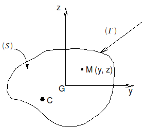
Figure 8 : general section.
If point \(c\) is the center of torsion (which by definition remains stationary when the beam is subjected to a twist), the field of displacement \(u(M)\) is given by [bib]:
\(u(M)\text{=}\left[\begin{array}{c}u\\ v\\ w\end{array}\right]\text{=}\left[\begin{array}{c}\frac{\partial {\theta }_{x}}{\partial x}x\\ 0\\ 0\end{array}\right]\wedge \left[\begin{array}{c}x\\ (y-{y}_{c})\\ (z-{z}_{c})\end{array}\right]\text{+}\left[\begin{array}{c}\frac{\partial {\theta }_{x}}{\partial x}\xi (y,z)\\ 0\\ 0\end{array}\right]\) \(\text{=}(\begin{array}{c}\frac{\partial {\theta }_{x}}{\partial x}\xi (y,z)\\ -\frac{\partial {\theta }_{x}}{\partial x}x(z-{z}_{c})\\ \frac{\partial {\theta }_{x}}{\partial x}x(y-{y}_{c})\end{array})\)
where \(\xi (y,z)\) is the warping function.
The law of HOOKE is written as:
\(\sigma \text{=}2\mu \varepsilon +(E-2\mu )\mathrm{Trace}(\varepsilon )I\)
where \(I\) is the unit matrix and the strain tensor is \(\varepsilon \text{=}\frac{1}{2}(\text{grad}(u)\text{+}{}^{T}\text{}\text{grad}(u))\)
By neglecting second-order terms, in \(\frac{{\partial }^{2}{\theta }_{x}}{\partial {x}^{2}}\), we end up with:
\(\sigma \text{=}\mu \frac{\partial {\theta }_{x}}{\partial x}\left[\begin{array}{ccc}0& \frac{\partial \xi }{\partial y}-z& \frac{\partial \xi }{\partial z}+y\\ \frac{\partial \xi }{\partial y}-z& 0& 0\\ \frac{\partial \xi }{\partial z}+y& 0& 0\end{array}\right]\) \(\text{=}\mu \frac{\partial {\theta }_{x}}{\partial x}\left[\begin{array}{ccc}0& \frac{\partial \varphi }{\partial z}& -\frac{\partial \varphi }{\partial y}\\ \frac{\partial \varphi }{\partial z}& 0& 0\\ -\frac{\partial \varphi }{\partial y}& 0& 0\end{array}\right]\) [10]
We set: \(\varphi (y\text{,}z)\) constraint function. It should be noted that the equilibrium relationship \(\text{div}s=0\) is then verified. By deriving, we obtain:
\(\begin{array}{c}\frac{{\partial }^{2}\varphi }{\partial {y}^{2}}\text{=}-\frac{{\partial }^{2}\xi }{\partial z\partial y}-1\\ \frac{{\partial }^{2}\varphi }{\partial {z}^{2}}\text{=}\frac{{\partial }^{2}\xi }{\partial y\partial z}-1\text{.}\end{array}\)
By adding the two equations, we end up with:
\(\Delta \varphi \text{=}\text{-}2\) [11]
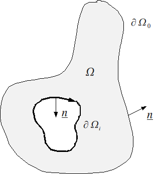
It remains to establish the boundary conditions. We note \(n\) the normal directed outside the border (\(\Gamma\)) which can be multiplied by the following:
Without external loading, we need to have \(\sigma \otimes n=0\), which can be written as:
\(\mu \frac{\partial {\theta }_{x}}{\partial x}\left[\begin{array}{c}\frac{\partial \varphi }{\partial z}{n}_{y}-\frac{\partial \varphi }{\partial y}{n}_{z}\\ 0\\ 0\end{array}\right]=0\) where \({n}_{y}\) and \({n}_{z}\) are the two components of normal.
This writing can thus be in the form \(n\wedge \text{grad}\varphi =0\) which implies that the vectors \(n\) and \(\text{grad}j\) are collinear. So it follows that \(\varphi (y,z)\) is constant on each connected component of the border (\(\Gamma\)). For example, we can impose that \(\varphi (y,z)\) be zero on the outer contour:
\(\varphi =0\) out \(\partial {\Omega }_{0}=\Gamma\)
\(\varphi ={\varphi }_{i}\) out \(\partial {\Omega }_{i}\)
In the case where the behavior sections of the holes, the \({\varphi }_{i}\) constants are undetermined. To solve the complete problem, equations must be added. These are obtained from the circulation of the warping function on each closed contour. The following conditions are obtained:
\({\oint }_{\partial {\Omega }_{i}}\frac{\partial \varphi }{\partial n}\text{dl}=\mathrm{2A}(\partial {\Omega }_{i})\)
where \(A(\partial {\Omega }_{i})\) is the area surrounded by border \((\partial {\Omega }_{i})\). These conditions are reduced to classical conditions of imposed flow (where \(l(\partial {\Omega }_{i})\) represents the length of the \((\partial {\Omega }_{i})\) border):
\(\frac{\partial \varphi }{\partial \underline{n}}=\frac{\mathrm{2A}(\partial {\Omega }_{i})}{l(\partial {\Omega }_{i})}\)
Finally, the problem to be solved is written as:
\(\Delta \varphi =-2\) out of \(\Omega\)
\(\varphi =0\) out of \(\partial {\Omega }_{0}=\Gamma\)
\(\varphi ={\varphi }_{i}\) out of \((\partial {\Omega }_{i})\)
\(\frac{\partial \varphi }{\partial \underline{n}}=\frac{\mathrm{2A}(\partial {\Omega }_{i})}{l(\partial {\Omega }_{i})}\)
Once this problem has been solved, the torsional constant is obtained by:
\(\mathrm{CT}=2{\int }_{\Omega }\varphi \text{ds}+2\sum _{i=1}^{n-1}{\varphi }_{i}A(\partial {\Omega }_{i})\).
3.2. Calculating the torsional constant in MACR_CARA_POUTRE#
This calculation is carried out in MACR_CARA_POUTRE by solving a thermal problem. To do this, the user must specify to MACR_CARA_POUTRE the mesh group that defines the outer edge, and if the section has holes, the mesh groups that define the outline of each of them.
A linear thermal problem (THER_LINEAIRE) is then solved on a plane mesh of the section in order to find the function \(j\). First of all, we place ourselves in the main inertia frame of reference (CREA_MAILLAGE), based on the coordinates of the center of gravity and the orientation of the main frame of reference calculated previously.
We then define the boundary conditions in AFFE_CHAR_THER:
Source term is —2
The temperature of the outer edge is set and is 0 (TEMP_IMPO)
If the section has holes (presence of one or more groups of cells defining them):
On each cell group defining a hole, the temperature is constant (TEMP_UNIF)
The flow is equal to 2 times the area of the hole divided by the length of its edge. These quantities are calculated previously.
The calculation of \(\mathit{JX}\) is done in POST_ELEM by the keyword CARA_TORSION of the keyword factor CARA_POUTRE. In this case, we calculate the integral of \(j\) on each element, (option CARA_TORSION on plane thermal elements), then we perform the sum on all the elements.
Example:
Let’s go back to the example of the rectangular section [§1.1.4]. The shear coefficients obtained are:
LIEU |
|
\(\mathit{JX}\) (Aster) |
all |
9.9805E-08 |
9.9681E-08 |
3.3. Calculation of the radius of torsion in any section#
The radius of torsion is calculated by calculating the stress function on the mesh of the section. \(\mathrm{Rt}\) is added to the table produced by MACR_CARA_POUTRE [U4.42.02].
Solving a stationary thermal problem with unknown \(j\) makes it possible to determine the torsional constant and the shear stresses.
The determination of the radius of torsion \(\mathrm{Rt}\) is the resolution of: \(\mathrm{Rt}=\mathrm{grad}(\varphi )\mathrm{.}n\) (where \(n\) represents the normal vector external to the considered edge of the section).
\(\mathrm{Rt}\) varies along the outer contour; in fact, for any section, the shear due to twisting varies at the edge. We choose to take the value of \(\mathrm{Rt}\) leading to the maximum shear on the outer edge, that is to say the maximum value of \(\mathrm{Rt}\) (in absolute value) on the outer contour.
In addition, if the section is honeycombed, we have several « several radii of torsion »: \(\mathrm{Rt}=2\ast A(k)/L(k)\) (where \(A(k)\) represents the area of the cell \(k\) and \(L(k)\) its perimeter). If we are simply looking for the maximum shear value, we must take the maximum of the \(\mathrm{Rt}\) values obtained on the outer edge and on the cells.
The radius of twist is determined in MACR_CARA_POUTRE by python commands only. During the execution of MACR_CARA_POUTRE the command POST_ELEM is called, a new parameter \(\mathrm{Rt}\) is therefore created for this command.
3.4. Torsion constant for circular and rectangular sections#
Simplified expressions for these two types of sections are described here. The calculation of the torsional constants is then performed directly in AFFE_CARA_ELEM.
For the circular section the previous expressions remain valid. By taking a twist function of the form \(\varphi (y\text{,}z)\text{=}\frac{1}{2}({R}^{2}-{x}^{2}-{y}^{2})\) we actually find:
\(\mathrm{CT}={I}_{p}=\frac{\pi }{2}({R}_{0}^{4}-{R}_{1}^{4})\)
For the rectangular section, the calculation is naturally more complex but can be done by choosing a function that effectively cancels at the edges, of the form:
\(\varphi (y\text{,}z)\text{=}\sum _{i=0}^{\text{+}\infty }\sum _{j=0}^{\text{+}\infty }{A}_{\text{ij}}\text{cos}\left[(\mathrm{2i}+1)\frac{\pi y}{{h}_{y}}\right]\text{cos}\left[(\mathrm{2j}+1)\frac{\pi z}{{h}_{z}}\right]\)
The resolution leads to a torsional constant which is written as:
\(\mathrm{CT}=\frac{{h}_{y}^{3}{h}_{z}^{3}}{{h}_{y}^{2}+{h}_{z}^{2}}c(\frac{{h}_{y}}{{h}_{z}})={h}_{y}{h}_{z}^{3}\left[\frac{c(\frac{{h}_{y}}{{h}_{z}})}{1+{(\frac{{h}_{z}}{{h}_{y}})}^{2}}\right]\) [12]
where \(c(\frac{{h}_{y}}{{h}_{z}})\) is expressed in the form of a series that takes the following values:
\(\begin{array}{cccccc}\frac{{h}_{y}}{{h}_{z}}& 1& 2& 4& 8& +\infty \\ c(\frac{{h}_{y}}{{h}_{z}})& \mathrm{0,}\text{281}& \mathrm{0,}\text{286}& \mathrm{0,}\text{299}& \mathrm{0,}\text{312}& 1/3\end{array}\)
In fact, Code_Aster uses a simplified formula (ref. [bib]) for the solid rectangular section which is written as:
\(\mathrm{CT}=\frac{{h}_{y}{h}_{z}^{3}}{16}(\frac{16}{3}-3.36\frac{{h}_{z}}{{h}_{y}}+0.280{(\frac{{h}_{z}}{{h}_{y}})}^{5})\) [13]
It is valid if \({h}_{y}>{h}_{z}\); in the other case it is enough to exchange the respective places of \({h}_{y}\) and \({h}_{z}\). The agreement between the two expressions is very good as shown in the following table:
\(\frac{{h}_{y}}{{h}_{z}}\) |
1 |
2 |
2 |
4 |
4 |
8 |
∞ |
\(\frac{\mathit{JX}}{{h}_{y}{h}_{z}^{3}}\) according to [eq] |
0.1405 |
0.1405 |
0.2288 |
0.2814 |
0.3072 |
1/3 |
|
\(\frac{\mathit{JX}}{{h}_{y}{h}_{z}^{3}}\) according to Aster [eq] |
0.1408 |
0.1408 |
0.2289 |
0.2809 |
0.3071 |
1/3 |
For the hollow rectangular beam, there is an approximate solution that can be written (ref. [bib] and [bib]):
\(\mathit{JX}\mathrm{=}\frac{2{\text{ep}}_{y}{\text{ep}}_{z}{({h}_{y}\mathrm{-}{\text{ep}}_{y})}^{2}{({h}_{z}\mathrm{-}{\text{ep}}_{z})}^{2}}{{h}_{y}{\text{ep}}_{y}\mathrm{-}{\text{ep}}_{y}^{2}+{h}_{z}{\text{ep}}_{z}\mathrm{-}{\text{ep}}_{z}^{2}}\)
with the notations of [Figure]: section in plane \((\mathrm{0,}y,z)\).
3.5. The effective torsional radius#
The effective torsional radius \({R}_{T}\) makes it possible to calculate the maximum transverse torsional shear stress \({\sigma }_{{T}_{M}}\) as a function of the torsional moment. On this subject, you can consult the editorial staff of MASSONET on this aspect (ref. [bib]). So we have:
\({\sigma }_{{T}_{M}}\mathrm{=}{M}_{x}\frac{{R}_{T}}{\mathit{JX}}\)
In the case of circular cylinders, \({R}_{T}\) is equal to the radius (external if it is a tube) of the section.
For rectangular sections, the problem is much more complex. Code_Aster imposes the radius of torsion of the solid section by:
\({R}_{T}\mathrm{=}\frac{\mathit{JX}4(3{h}_{y}+1.8{h}_{z})}{{h}_{y}^{2}+{h}_{z}^{2}}\)
This approximate expression remains valid if the beam is not too flattened. DHATT and BATOZ (ref. [bib]) give an expression with a wider field of validity, but in reality it is from a harmonious point of view a series whose numerical values are given by MASSONET (ref. [bib]).
For the hollow rectangular beam, Code_Aster imposes an expression that is only valid if the wall is thin and of constant \({\mathrm{ep}}_{z}\) thickness, i.e.:
\({R}_{T}\text{=}\frac{\mathit{JX}}{{\text{ep}}_{z}({h}_{y}\mathrm{-}2{\text{ep}}_{y})({h}_{z}\mathrm{-}2{\text{ep}}_{z})}\)
It is an « adaptation » of the formula:
\({R}_{T}\mathrm{=}\frac{\mathit{JX}}{2eA}\)
where \(e\) is the wall thickness (constant) and \(A\) is the area contained within the mean line. This last expression is known as the first formula in BREDT (see Ref. [bib] and [bib]).