2. Shear coefficients and the shear center

The aim is to evaluate the \({A}_{y}=\frac{1}{{k}_{y}},{A}_{z}=\frac{1}{{k}_{z}}\) coefficients used in Timoshenko beam models taking into account shear deformations. For the EULER beams, these coefficients do not intervene [U4.42.01 §7.4.2] and [R3.08.01 §2.3.1]. These coefficients are obtained for linear elastic behavior.

In the case of any sections, the shear coefficients are to be provided by the user in AFFE_CARA_ELEM, if the element chosen is a TIMOSHENKO beam (models POU_D_T, POU_D_TG and POU_D_TGM).

In the case of circular or rectangular sections, shear coefficients are calculated by [§2.1] analytical methods.

In all cases, they can be calculated by MACR_CARA_POUTRE, based on the plane mesh of the section. The numerical method used is shown in [§2.3]. This method applies to any sections (of homogeneous and isotropic material). In appendix 2, an extension of this method is described in the case of a network of parallel beams held between two rigid floors.

The position of the center of torsion (or center of shear) can only be obtained by numerical methods (cf. [§2.3]). For rectangular and circular sections, as for all sections with 2 planes of symmetry, the center of torsion coincides with the center of gravity of the section.

2.1. Analytical methods

Three analytical methods for calculating shear coefficients applicable to any cross-sections are described.

The first two methods differ in the definition they propose of the shear coefficient, but are based on the same hypothesis which consists in postulating the shape of the distribution of shear stresses in the section.

2.1.1. Shear distribution hypothesis: JOURAWSKI formula

For example, consider the case of a beam with a straight section \(S\), subjected to a shear force \({V}_{y}={\int }_{s}{\sigma }_{\mathrm{xy}}\mathrm{dS}\). We write the balance of a prismatic part of the beam, between the straight sections \({S}_{x}\) and \({S}_{x+a}\) and between the plane of section located at the ordinate \(y\) and \({y}_{\mathrm{max}}\) (ref. [bib]). The forces acting on this part of the beam are the vectors constrained on faces \({S}_{x}\) and \({S}_{x+a}\), and those acting on the face located in \(y\).

Figure 6 : Beam section.

Applying the resultant theorem, we get:

\(\begin{array}{cc}{\int }_{{S}_{x+a}}{\sigma }_{\text{xx}}(x,y\text{'},z)\mathrm{dy}\text{'}\text{dz}-{\int }_{{S}_{x}}{\sigma }_{\text{xx}}(x,y\text{'},z)\mathrm{dy}\text{'}\text{dz}& \text{=}N(x+a,y)-N(x,y)\\ & \text{=}{\int }_{x}^{x+a}{\int }_{\frac{-b(y)}{2}}^{\frac{b(y)}{2}}{\sigma }_{\text{xy}}(\alpha ,y,z)d\alpha \text{dz}\end{array}\)

To evaluate the term on the right, JOURAWSKI proposed to consider only the mean of the shears following z:

\({\stackrel{ˉ}{\sigma }}_{\text{xy}}(x,y)=\frac{1}{b(y)}{\int }_{\text{-}\frac{b}{2}}^{\frac{b}{2}}{\sigma }_{\text{xy}}(x,y,z)\text{dz}\)

then

\({\int }_{x}^{x+a}{\int }_{-\frac{b(y)}{2}}^{\frac{b(y)}{2}}{\sigma }_{\text{xy}}(\alpha ,y,z)d\alpha \text{dz}={\int }_{x}^{x+a}b(y){\stackrel{ˉ}{\sigma }}_{\text{xy}}(\alpha ,y)d\alpha\)

and by tending \(a\) to \(0\),

\(\frac{\partial N}{\partial x}=b(y){\stackrel{ˉ}{\sigma }}_{\text{xy}}(x,y)\)

The beam equilibrium equations and the distribution of flexural stresses (in elasticity) give:

\(N(x,y)={\int }_{{S}_{x}}^{}{\sigma }_{\text{xx}}(x,y,z)\text{dydz}={\int }_{{S}_{x}}^{}\frac{{M}_{z}(x)\text{.}y}{{I}_{z}}\text{dydz}\)

\(=\frac{{M}_{z}(x)}{{I}_{z}}m(y)\text{avec}m(y)={\int }_{y}^{{y}_{\text{max}}}t\text{}b(t)\text{}\text{dt}\)

therefore

\({\stackrel{ˉ}{\sigma }}_{\text{xy}}(\text{x,y})\text{=}\frac{m(y)}{{I}_{z}b(y)}\frac{\partial {M}_{z}}{\partial x}=\frac{m(y)}{{I}_{z}b(y)}{V}_{y}\)

The shear distribution following \(y\) is therefore given by the formula for JOURAWSKI:

\({\stackrel{ˉ}{\sigma }}_{\text{xy}}(\text{x,y})\text{=}\frac{m(y)}{{I}_{z}b(y)}{V}_{y}\text{avec}m(y)\text{=}{\int }_{y}^{{y}_{\text{max}}}t\text{}b(t)\text{}\text{dt}\) [1]

in accordance with [U4.24.01], with the notations in [Figure]. The quantity \(m(y)\) represents the static moment of the section portion (shaded) between \(y\) and \({y}_{\mathrm{max}}\):

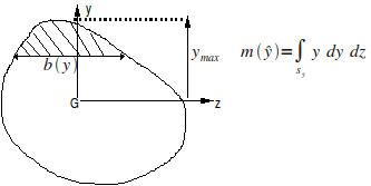
Figure 7 : beam section

This distribution does indeed verify the boundary conditions following \(y\) of the three-dimensional problem: the shear is indeed zero on the lower and upper fibers (\(y={y}_{\text{min}}\), or \(y={y}_{\text{max}}\)). But it only takes into account the average of the shears following \(z\).

Applying this formula to a solid rectangular section, we find a parabolic distribution following \(y\). Applying it to a circular cross-section beam, we find a parabolic distribution in y and in \(z\), which varies more slowly along \(z\) than along \(y\).

This remains valid for the other full sections. For sections with holes, be careful to consider only the material when calculating \(b(y)\).

2.1.2. TIMOSHENKO method

Originally, TIMOSHENKO (ref. [bib]) proposed a simple definition of the shear coefficient, as being the ratio between the mean transverse shear stress in the section noted \({\stackrel{ˉ}{\sigma }}_{\text{CT}}\) and its maximum value \(({\sigma }_{{\mathrm{CT}}_{\mathrm{Max}}})\). Because we always have the best effort by:

\(V\text{=}{\int }_{s}{\sigma }_{\text{CT}}\text{dS}\) [2]

we deduct:

. \({\stackrel{ˉ}{\sigma }}_{\text{CT}}\text{=}\frac{V}{S}\)

Knowing that TIMOSHENKO proposes to write:

\(k\text{=}\frac{{\stackrel{ˉ}{\sigma }}_{\text{CT}}}{{\sigma }_{{\text{CT}}_{\text{Max}}}}\) [3]

To determine \(k\), simply express the shear force \(V\text{=}{\int }_{s}{\sigma }_{\text{CT}}\text{dS}\) [eq] as a function of \({\sigma }_{{\mathrm{CT}}_{\mathrm{Max}}}\). In the general case of any sections, there will naturally be two coefficients \({k}_{y}\) and \({k}_{z}\), for each of the two main axes.

\({\sigma }_{{\mathrm{CT}}_{\mathrm{Max}}}\) is yet to be determined. For this, TIMOSHENKO makes an assumption about the distribution of transverse shear stresses: the transverse shear stress has a parabolic distribution in the direction of the shear force that produces it, with its maximum value at the center and zero values at the edges. This is true according to the JOURAWSKI formula for a rectangular section. By extension, the method extends this parabolic distribution hypothesis to any section

This method is not applied in*Code_Aster* except for hollow rectangular sections. The « energetic » method is used in other cases.

2.1.3. « Energetic » method

In reality, the definition proposed by TIMOSHENKO proves to be little used in practice today; we prefer a formulation based on the internal energy due to shear in the section. This one is written:

\({U}_{\text{CT}}\text{=}{\int }_{s}\frac{1}{2}\frac{{\sigma }_{{\text{CT}}^{2}}}{G}\text{dS}\)

where \(G\) is the shear modulus (equal to \(m\)).

The new definition of shear coefficient is sometimes attributed to MINDLIN and is expressed by:

\({U}_{\text{CT}}\text{=}\frac{1}{2}\frac{{V}^{2}}{k\text{SG}}\) [4]

Therefore, by substitution, the shear coefficient is thus defined for a homogeneous material section by:

\(k\text{=}{\frac{\left[{\int }_{s}{\sigma }_{\text{CT}}\text{dS}\right]}{S{\int }_{s}{\sigma }_{{\text{CT}}^{2}}\text{dS}}}^{2}=\frac{{V}^{2}}{S{\int }_{s}{\sigma }_{{\text{CT}}^{2}}\text{dS}}\) [5]

By making an assumption about the distribution of stress in the section, we can thus estimate the value of \(k\). From the formula for JOURAWSKI [eq], the previous expression can be written as [bib]:

\(k\text{=}\frac{{I}^{2}}{S{\int }_{S}^{}\frac{{m}^{2}(y)}{{b}^{2}(y)}\text{dS}}\) [6]

2.1.4. COWPER method

It is also possible to take into account three-dimensional effects to determine the coefficient \(k\); various formulations have been proposed, in particular by COWPER [bib] and taken up by BLEVINS [bib], based on the resolution of the three-dimensional Saint-Venant problem.

In this case, the coefficient \(k\) is a function of the coefficient of POISSON, generally a first-order approximation. COWPER uses the three-dimensional equations of elasticity in the dynamic case to propose an expression for \(k\) giving good results in statics and dynamics at low frequency. The approximation that makes it possible to arrive at the proposed formula consists in considering a stress distribution that is not parabolic, but resulting from the static problem (solved analytically) of the cantilever beam loaded transversely at its free end. It should be noted that the distribution obtained is strictly identical to the problem with a uniformly distributed transverse loading.

2.2. Special case of rectangular and circular sections

A distinction is made between solid beams and tubes.

For the solid rectangular section, the shear coefficient is determined by the method based on internal shear energy with parabolic stress distribution:

\({k}_{y}\text{=}\frac{{I}_{z}^{2}}{S{\int }_{S}^{}\frac{{m}_{z}^{2}(y)}{{b}_{{}_{z}}^{2}(y)}\text{dy}}\) [7]

When applied to the rectangular section, we get \({k}_{y}\text{=}{k}_{z}\text{=}\frac{5}{6}\). Note that this value also corresponds to the COWPER method when the POISSON coefficient is taken to be equal to zero.

For the rectangular tube, Code_Aster uses the TIMOSHENKO method which leads to \({k}_{y}\text{=}{k}_{z}\text{=}\frac{2}{3}\). In the case of beams with a full circular section, the energetic method that leads to \({k}_{y}\text{=}{k}_{z}\text{=}\frac{9}{10}\) is used. This value is also obtained by the COWPER method when the coefficient of POISSON is equal to \(\frac{1}{2}\).

For circular tubes, a distinction is made between thin-walled tubes and thick-walled tubes. If we note \(m\text{=}\frac{{r}_{i}}{{r}_{e}}\) the ratio of the internal radius to the external radius, a tube is thin-walled when \(m>0.9\), otherwise it is thick-walled.

The shear coefficient of the thin-walled circular tube is given by the method of COWPER, considering that \(m=1\) and for a zero coefficient of POISSON, that is to say \({k}_{y}\text{=}{k}_{z}\text{=}\frac{1}{2}\).

For thick-walled circular tubes, a formula similar to the COWPER method is used, which is written as: \(k\text{=}\frac{1}{\mathrm{1,}\text{093}\text{+}\mathrm{0,}\text{634}m\text{+}\mathrm{1,}\text{156}{m}^{2}-\mathrm{0,}\text{905}{m}^{3}}\)

Note that this formula does not ensure continuity with the limiting cases of the solid cylinder (\(m=0\)) and the cylinder with an infinitely thin wall (\(m=1\)).

If the previous choices (made by AFFE_CARA_ELEM in the case of circular and rectangular sections) are not appropriate, it is still possible to calculate shear coefficients numerically using MACR_CARA_POUTRE, whose method is specified in the following §.

2.3. Numerical method for calculating shear coefficients and shear center

2.3.1. Calculation of shear coefficients:

This method is based on [bib], page 62. It allows the simultaneous determination of shear constants and the center of torsion. It is implemented in MACR_CARA_POUTRE, based on a plane mesh of the section. It currently only works for homogeneous and isotropic sections (for non-homogeneous sections, the method is similar [bib] but not available in Code_Aster).

As for the energetic method, for a shear force \(V\), we compare the internal energy \({U}_{1}\) due to shear in the section with the energy U2associated with the model of MINDLIN:

\({U}_{1}\text{=}{\int }_{s}\frac{1}{2}\frac{{\sigma }_{\text{xy}}^{2}+{\sigma }_{\text{xz}}^{2}}{G}\text{dS}={U}_{2}=\frac{1}{2}\frac{{V}_{z}^{2}}{{k}_{z}\text{SG}}\)

The shear coefficient is expressed as: \({k}_{z}\text{=}\frac{1}{2}\frac{{V}_{z}^{2}}{{\text{SGU}}_{1}}\)

It is therefore necessary to calculate \({U}_{1}\) and therefore the shear stresses (in elasticity) in the section in order to estimate the value of \(k\). We place ourselves in the main inertia coordinate system \((G,y,z)\), and we assume that the beam is only subjected to a shear force \({V}_{z}\). The result is that:

\(\begin{array}{}{\sigma }_{\text{xx}}=z\frac{{M}_{y}(x)}{{I}_{y}}\\ \frac{\partial {\sigma }_{\text{xx}}}{\partial x}=z\frac{{V}_{z}}{{I}_{y}}\end{array}\)

Equilibrium equations allow you to write:

\(\frac{\partial {\sigma }_{\text{xx}}}{\partial x}+\frac{\partial {\sigma }_{\text{xy}}}{\partial y}+\frac{\partial {\sigma }_{\text{xz}}}{\partial z}=0=\frac{\partial {\sigma }_{\text{xy}}}{\partial y}+\frac{\partial {\sigma }_{\text{xz}}}{\partial z}+z\frac{{V}_{z}}{{I}_{y}}\)

On the other hand, the kinematics of the flexion/shear beam is:

\(\begin{array}{}u(x,y,z)=u(x)+z{\theta }_{y}(x)+\tilde{u}(y,z)\\ v(x,y,z)=0\\ w(x,y,z)=w(x)\end{array}\)

\(\tilde{u}(y,z)\) representing axial displacement due to warping of the section. The deformations are written as:

\(\begin{array}{}{\varepsilon }_{\text{xx}}=\frac{\partial u(x)}{\partial x}+z\frac{\partial {\theta }_{y}(x)}{\partial x}\\ 2{\varepsilon }_{\text{xy}}=\frac{\partial \tilde{u}(y,z)}{\partial y}\\ 2{\varepsilon }_{\text{xz}}={\theta }_{y}(x)+\frac{\partial \tilde{u}(y,z)}{\partial z}+\frac{\partial w(x)}{\partial x}\end{array}\)

Using the linear elasticity behavior relationship, the constraints are written as:

\(\begin{array}{}{\sigma }_{\text{xy}}=2\mu {\varepsilon }_{\text{xy}}=\mu \frac{\partial \tilde{u}(y,z)}{\partial y}\\ {\sigma }_{\text{xz}}=2\mu {\varepsilon }_{\text{xz}}=\mu ({\theta }_{y}(x)+\frac{\partial \tilde{u}(y,z)}{\partial z}+\frac{\partial w(x)}{\partial x})\end{array}\)

The shear components therefore verify:

\(\frac{\partial {\sigma }_{\text{xy}}}{\partial z}-\frac{\partial {\sigma }_{\text{xz}}}{\partial y}=0\)

This relationship makes it possible to introduce the stress function \({\psi }_{z}\) such that the shear stresses in the section are written as:

\(\begin{array}{}{\sigma }_{\text{xy}}=\mu \frac{\partial {\psi }_{z}}{\partial y}\\ {\sigma }_{\text{xz}}=\mu \frac{\partial {\psi }_{z}}{\partial z}\end{array}\)

The equilibrium equation then makes it possible to obtain function \({\psi }_{z}\) by solving a quasi‑harmonic problem which is written as:

\(\begin{array}{}G\Delta {\psi }_{z}+f=0\text{dans}S\text{avec}f=\frac{{\mathrm{zV}}_{z}}{{I}_{y}}\\ G\frac{\partial {\psi }_{z}}{\partial n}=0\text{sur}\partial S\\ {\psi }_{z}=0\text{en un point}\end{array}\)

This makes it possible to calculate \({\psi }_{z}\) and then the shears. In practice, in MACR_CARA_POUTRE, THER_LINEAIRE is used to solve the problem, equating \({\psi }_{z}\) to temperature. We choose \(V=1\) and \(G=1\) (\(G\) is no longer involved in the expression of the shear coefficient). The boundary conditions for this stationary thermal problem are:

• source \(f\) equal to \(\frac{{\text{zV}}_{z}}{{I}_{y}}\)

• zero flow on \(\partial S\)

• zero temperature at a point of \(S\)

We can then determine \({U}_{1}^{z}={\int }_{s}\frac{1}{2}\frac{{\sigma }_{\text{xy}}^{2}+{\sigma }_{\text{xz}}^{2}}{G}\text{dS}=\frac{1}{2}{\int }_{s}G{(\nabla {\psi }_{z})}^{2}\text{dS}\) by an elementary calculation on all the elements of the section, with the option “CARA_CISA” (calculation of the gradient), then summation on these elements. We then calculate \({k}_{z}\text{=}\frac{1}{2}\frac{{V}_{z}^{2}}{{\text{SGU}}_{1}^{z}}\)

The same calculation is done with \({V}_{y}=1\) to determine \({k}_{y}\text{=}\frac{1}{2}\frac{{V}_{y}^{2}}{{\text{SGU}}_{{}_{1}}^{y}}\)

The result provided is \({A}_{y}=\frac{1}{{k}_{y}},{A}_{z}=\frac{1}{{k}_{z}}\).

2.3.2. Calculating the coordinates of the shear center

Shear center \(C\) is the point in the section where shear stresses due to shear force cause zero torsional moment. This point is also called the center of torsion, because it remains fixed when the section is only subjected to a torsional moment.

The torsional moment with respect to point \(G\) is equal to \({M}_{\text{xG}}\text{=}{\int }_{s}({\sigma }_{\text{xz}}\text{.}y-{\sigma }_{\text{xy}}\text{.}z)\text{dS}\):

The torsional moment with respect to the sought point \(C\) is:

\({M}_{\text{xC}}\text{=}{\int }_{s}({\sigma }_{\text{xz}}\text{.}(y-{y}_{c})-{\sigma }_{\text{xy}}(z-{z}_{c}))\text{dS}={M}_{\text{xG}}-{y}_{c}{V}_{z}+{z}_{c}{V}_{y}\)

To determine the coordinates of the shear center, we use the previous calculation [bib]:

From the shear stresses determined for \(V=1\) and \({V}_{y}=0\), we calculate: \({M}_{{}_{\text{xG}}}^{z}\text{=}{\int }_{s}({\sigma }_{\text{xz}}\text{.}y-{\sigma }_{\text{xy}}\text{.}z)\text{dS}\)

We get: \({y}_{c}=\frac{{M}_{{}_{\text{xG}}}^{z}}{{V}_{z}}={M}_{{}_{\text{xG}}}^{z}\)

For \(V=1\) and \({V}_{y}=0\), we get: \({z}_{c}=-\frac{{M}_{\mathrm{xG}}^{y}}{{V}_{y}}=-{M}_{{}_{\text{xG}}}^{y}\)

2.3.3. example

Let’s go back to the example of the rectangular section [§1.1.4].

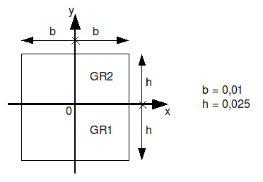
The shear coefficients obtained are identical to the analytical value (6/5).

\(\mathrm{LIEU}\)	\(\mathrm{AY}\)	\(\mathrm{AZ}\)		\(\mathrm{EY}\)	\(\mathrm{EZ}\)
all	1.20E+00	1.20E+00	—8.72E-19	3.16E—18

The components of the vector \(\mathrm{CG}=(\mathrm{EY},\mathrm{EZ})\) expressed in the main coordinate system \((G,y,z)\) are zero: the shear and torsional center is effectively confused with the center of gravity.

2.4. Calculation of the shear coefficients of a network

The method described in Appendix 2 makes it possible to calculate shear coefficients for a beam equivalent to a set of parallel beams embedded on a rigid floor and embedded or hinged on another.