5. Bibliography

[1] BATOZ J.L. & DHATT G.: « Modeling structures using finite elements. Volume 2, beams and plates ». HERMES, Paris, 1990

[2] BLEVINS R.D.: « Formulas for natural frequency and mode shape. » Van Nostrand Reinhold, New York, 1979.

[3] COWPER G.R.: « The shear coefficient in Timoshenko’s beam theory. » J. of Applied Mechanics, June 1966, pp 335-340.

[4] HSU Y.W.: « The shear coefficient of beams of circular cross section ». J. of Applied Mechanics, March 1975, pp 226-228.

[5] MASSONET C. & CESCOTTO S.: « Mechanics of materials ». De boeck University, Brussels, 1994.

[6] PILKEY W.D.: « Formulas for Stress, Strain and Structural Matrixes. » Wiley & Sons, New York, 1994.

[7] REISSNER E. & TSAI W.T.: « On the determination of the centers of twist and of shear for cylindrical shell beams. » J. of Applied Mechanics, December 1972, pp1098-1102.

[8] BAMBERGER Y.: Material Resistance Course - National School of Bridges and Roads. 1994.

[9] TIMOSHENKO S. Material Strength - Dunod 1968

[10] Document [U4.24.01]: Operator AFFE_CARA_ELEM

[11] VOLDOIRE F: « Material strength elements. Tutorials from ENPC ». Rating EDF/MMN HI-74/96/002/0

Description of document versions:

Version Aster	Author (s) Organization (s)	Description of changes
7.4	J.M. Proix, N. Laurent, P. Hemon, G. Bertrand EDF -R&D/ AMA, IAT St Cyr, CS-SI
8.5	J.M.Proix, EDF -R&D/ AMA	Unit correction page 24, Sheet REX 10783
10	Jean-Luc FLÉJOU, EDF -R&D/ AMA	Formatting, correction of formulas, Sheet REX 16337
12.4	Jean-Luc FLÉJOU, EDF -R&D/ AMA	Suppression POU_C_T (23282)

Determination of the torsional constant for multiply-related border sections

Consider an elastic, isotropic beam of length \(L\) and any cross section \(\Omega\) that can not simply be connected. We note \(\partial {\Omega }_{0}\) the outer outline of \(\Omega\) and \(\partial {\Omega }_{1}\), for \(i=\mathrm{1...n}-1\), the possible inner contours. Its total border is noted \(\partial \Omega =\underset{i=0}{\overset{n-1}{\cup }}\partial {\Omega }_{i}\).

We choose the \({\underline{x}}_{1}\) axis according to the line of the centers of gravity of the straight sections. To simplify the demonstration, it is assumed that the center of torsion is confused with the center of gravity, which makes it possible to decouple the effects of torsion and bending. The axes \({\underline{x}}_{2}\) and \({\underline{x}}_{3}\) are chosen according to the main directions of inertia.

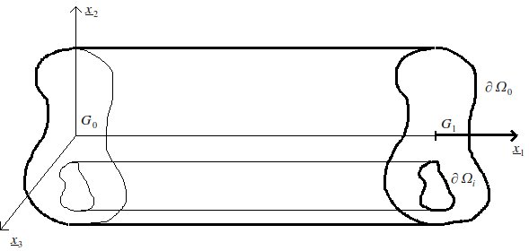
Figure 9 : Beam with any cross section.

The beam is loaded onto its section \({x}_{1}=L\) by a torsional moment \({\underline{M}}_{{G}_{1}}={M}_{t}{\underline{x}}_{1}\).

On the other hand, the lateral surface of the cylinder is not loaded and the volume forces are zero.

We immediately deduce that the twister of internal forces at point \({G}_{0}\) is \({\underline{M}}_{{G}_{0}}={M}_{t}{\underline{x}}_{1}\)

The elasticity problem posed above appears to be incompletely defined. Indeed, the boundary conditions on straight sections \({x}_{1}=L\) and \({x}_{1}=0\) are incomplete because we do not have a condition at each point, but on average. So, a priori, there are an infinity of solutions. The Saint-Venant hypothesis consists in looking for a solution such that the stress tensor is of the form:

\(\sigma =\left[\begin{array}{ccc}{\sigma }_{\text{11}}& {\sigma }_{\text{12}}& {\sigma }_{\text{13}}\\ {\sigma }_{\text{12}}& 0& 0\\ {\sigma }_{\text{13}}& 0& 0\end{array}\right]\)

The Saint-Venant principle is valid far from the application of forces sections. In fact, except in cases of particular loads, the four terms that are supposed to be zero are amortized exponentially with \({x}_{1}\).

To solve this elasticity problem, a stress formulation is chosen. The equations to be written are therefore those of balance and those of compatibility.

Balance equations \(\text{div}\sigma =\underline{0}\) lead to the following three scalar equations:

\({\partial }_{1}{\sigma }_{\text{11}}+{\partial }_{2}{\sigma }_{\text{12}}+{\partial }_{3}{\sigma }_{\text{13}}=0\) [14]

\(\begin{array}{}{\partial }_{1}{\sigma }_{\text{12}}=0\\ {\partial }_{1}{\sigma }_{\text{13}}=0\end{array}\) [15]

(with simplified notation:) \({\partial }_{i}{\sigma }_{\text{jk}}=\frac{\partial {\sigma }_{\text{jk}}}{\partial {x}_{i}}\)

The Beltrami equations, which take compatibility equations into account, are written as:

\(-\Delta {\sigma }_{\text{11}}-{\partial }_{\text{11}}{\sigma }_{\text{11}}=0\) [16]

\(-\Delta {\sigma }_{\text{12}}-\frac{1}{1+\nu }{\partial }_{\text{12}}{\sigma }_{\text{11}}=0\) [17]

\(-\Delta {\sigma }_{\text{13}}-\frac{1}{1+\nu }{\partial }_{\text{13}}{\sigma }_{\text{11}}=0\) [18]

\(-{\partial }_{\text{22}}{\sigma }_{\text{11}}+\nu \Delta {\sigma }_{\text{11}}=0\) [19]

\(-{\partial }_{\text{23}}{\sigma }_{\text{11}}=0\) [20]

\(-{\partial }_{\text{33}}{\sigma }_{\text{11}}+\nu \Delta {\sigma }_{\text{11}}=0\) [21]

The equations [eq], [eq] and [eq] show that \({\partial }_{\text{11}}{\sigma }_{\text{11}}\), \({\partial }_{\text{22}}{\sigma }_{\text{22}}=0\) and \({\partial }_{\text{33}}{\sigma }_{\text{11}}\) are solutions of a homogeneous linear system and therefore that \({\partial }_{\text{11}}{\sigma }_{\text{11}}={\partial }_{\text{22}}{\sigma }_{\text{11}}={\partial }_{\text{33}}{\sigma }_{\text{11}}=0\). With the equation [eq], we deduce only \({\sigma }_{11}={a}_{0}+{a}_{1}{x}_{1}+({b}_{1}{x}_{1}+{b}_{0}){x}_{2}+({c}_{1}{x}_{1}+{c}_{0}){x}_{3}\). Taking into account that we are treating the free twist problem, we will take \({\sigma }_{11}\) null from now on.

The equations [eq] and [eq] show that \({\sigma }_{12}\) and \({\sigma }_{13}\) do not depend on \({x}_{1}\). The equation [eq] is written as:

\({\partial }_{2}\left[{\sigma }_{\text{12}}+f({x}_{3})\right]={\partial }_{3}\left[-{\sigma }_{\text{13}}-g({x}_{2})\right]\)

where \(f\) and \(g\) are two arbitrary functions. Based on Schwartz’s theorem, there is \(\varphi ({x}_{\mathrm{2,}}{x}_{3})\) such as:

\(\{\begin{array}{c}{\partial }_{2}\varphi \text{=}\text{-}{\sigma }_{\text{13}}-f({x}_{2})\\ {\partial }_{3}\varphi ={\sigma }_{\text{12}}+g({x}_{3})\end{array}=\{\begin{array}{c}{\sigma }_{\text{12}}={\partial }_{3}\varphi -f({x}_{3})\\ {\sigma }_{\text{13}}\text{=}\text{-}{\partial }_{2}\varphi +g({x}_{2})\end{array}\)

The equations [eq] and [eq] give:

\(\{\begin{array}{c}{\partial }_{3}\Delta \varphi =0\\ {\partial }_{2}\Delta \varphi =0\end{array}\)

Be \(\Delta \varphi ={\partial }_{3}f-{\partial }_{2}f+K\)

where \(K\) is an integration constant. Since \(f\) and \(g\) are arbitrary, we will take them to be equally null. So the problem to be solved is a Laplacian problem: \(\Delta \varphi =K\) on \(\Omega\) then:

\(\sigma =\left[\begin{array}{ccc}0& {\partial }_{3}\varphi & -{\partial }_{2}\varphi \\ {\partial }_{3}\varphi & 0& 0\\ -{\partial }_{2}\varphi & 0& 0\end{array}\right]\)

It remains to write the boundary conditions, which will allow us to write conditions on \(\varphi \Omega\) for \(\varphi\) and on \(K\)

The boundary conditions are to be written all over the border. On sections right \({x}_{1}=L\) (and similarly in \({x}_{1}=0\)), we have:

\({\int }_{\Omega }{\sigma }_{\text{12}}\text{ds}=0\)

\({\int }_{\Omega }{\sigma }_{\text{13}}\text{ds}=0\)

\({\int }_{\Omega }{x}_{2}{\sigma }_{\text{13}}-{x}_{3}{\sigma }_{\text{12}}\text{ds}={M}_{t}\) [22]

Let \(\underline{n}\) be the normal outside of \(\partial \Omega\). We have \(\sigma \otimes n=0\). We pose \(\tau ={\sigma }_{\text{12}}{x}_{2}+{\sigma }_{\text{13}}{x}_{3}\). We can also write \(\tau ={\sigma }_{\text{12}}{x}_{2}+{\sigma }_{\text{13}}{x}_{3}\); \(\tau\) is called the tangential part of the constraint in the right section. Let \({N}_{i}\) be the current point on the \(\varphi \Omega\) outline for \(i=\mathrm{0,}\mathrm{...},n-1\). The condition, on the lateral surface, stated above, can be written \(\tau {\text{dN}}_{i}=\underline{0}\).

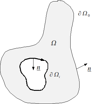
Figure 10 : Definition of normals

Thus, on the lateral surface of a beam, the tangential stress vector \(\tau\) is tangential to the outline.

• Equation \(\tau \wedge {\text{dN}}_{i}=\underline{0}\) leads to a condition that \(\varphi\) must meet on the contour: \(d\varphi =0\)

• The equation [eq] leads to \({M}_{t}={\int }_{\Omega }-{x}_{2}{\partial }_{2}\varphi -{x}_{3}{\partial }_{3}\varphi \text{ds}\) which can also be written as:

\({M}_{t}=2{\int }_{\Omega }\varphi \text{ds}+{\int }_{\partial \Omega }\varphi ({x}_{3}{\text{dx}}_{2}-{x}_{2}{\text{dx}}_{3})\)

So the problem to solve to get \(\varphi\) is:

\(\Delta \varphi =K\) out of \(\Omega\)

\(d\varphi =0\) out of \(\partial \Omega\)

with constraint \({M}_{t}=2{\int }_{\Omega }\varphi \text{ds}+{\int }_{\partial \Omega }\varphi ({x}_{3}{\text{dx}}_{2}-{x}_{2}{\text{dx}}_{3})\)

It remains to identify the torsional constant C. The law of torsional behavior of beams is: \({M}_{t}=\text{CG}\frac{\partial {\theta }_{x}}{\partial x}\) (cf. [§3]).

To solve the previous problem more easily, we ask \(\psi =\frac{\varphi }{C\frac{\partial {\theta }_{x}}{\partial x}}\) and \(K\text{=}-\mathrm{2C}\frac{\partial {\theta }_{x}}{\partial x}\), the problem to be solved then becomes:

\(\Delta \psi =-2\) out of \(\Omega\)

\(d\psi =0\) out of \(\partial \Omega\)

\({M}_{t}\text{=}-\mathrm{2C}\frac{\partial {\theta }_{x}}{\partial x}\left[{\int }_{\Omega }\psi \text{ds}+{\int }_{\partial \Omega }\psi ({x}_{3}{\text{dx}}_{2}-{x}_{2}{\text{dx}}_{3})\right]\)

With such a notation, we get \(C=2{\int }_{\Omega }\psi \text{ds}+{\int }_{\partial \Omega }\psi ({x}_{3}{\text{dx}}_{2}-{x}_{2}{\text{dx}}_{3})\)

Outline \(\partial \Omega\) consists of several contours: an outer contour \(\partial {\Omega }_{0}\) and \(n-1\) inner contours \(\partial {\Omega }_{i}\). Condition \(d\psi =0\) leads to the following \(n\) conditions: \(\psi ={\psi }_{i}\) out of \(\partial {\Omega }_{i}\) for \(i=\mathrm{0,}\mathrm{...},n-1\). \({\psi }_{i}\) are unknown constants. By noting that \(\varphi\), and therefore \(\psi\), is defined to one constant, we can set one of \({\psi }_{i}\). So we’ll take \({\psi }_{0}=0\). \({\psi }_{i}\) for \(i=\mathrm{0,}\mathrm{...},n-1\) remains to be determined.

To do this, we will study the warping of the right section of abscissa \({x}_{1}\). Recall that the stress tensor is written (cf. [§4]):

\(\sigma \text{=}G\frac{\partial {\theta }_{x}}{\partial x}\left[\begin{array}{ccc}0& \frac{\partial \xi }{\partial y}-z& \frac{\partial \xi }{\partial z}\text{+}y\\ \frac{\partial \xi }{\partial y}-z& 0& 0\\ \frac{\partial \xi }{\partial z}\text{+}y& 0& 0\end{array}\right]\) \(\text{=}G\frac{\partial {\theta }_{x}}{\partial x}\left[\begin{array}{ccc}0& \frac{\partial \psi }{\partial z}& -\frac{\partial \psi }{\partial y}\\ \frac{\partial \psi }{\partial z}& 0& 0\\ -\frac{\partial \psi }{\partial y}& 0& 0\end{array}\right]\)

Let’s say \(\underline{\tau }=\underline{\text{grad}}\psi \wedge {\underline{x}}_{1}\); \(\underline{\tau }\) is (except for one constant) the tangential part of the stress vector in the right section.

So we have: \(\underline{\text{grad}}\xi =\underline{\tau }-\underline{\text{GM}}\wedge {\underline{x}}_{1}\)

We circulate this equation along \(\partial {\Omega }_{i}\), we have:

\(0={\oint }_{\partial {\Omega }_{i}}\tau \text{dl}-{\oint }_{\partial {\Omega }_{i}}{x}_{3}{\text{dx}}_{2}-{x}_{2}{\text{dx}}_{3}\)

We used here the fact that the circulation of the gradient on a closed curve is zero.

Note that the first integral can be written in terms of the flow of \(\psi\) crossing \(\partial {\Omega }_{i}\). On the other hand, the second integral is equal to \(\mathrm{2A}(\partial {\Omega }_{i})\).

Finally, the problem is written:

\(\Delta \psi =-2\) out of \(\Omega\)

\(\psi =0\) out of \(\partial {\Omega }_{0}\)

\(\psi ={\psi }_{i}\) out of \(\partial {\Omega }_{i}\)

\({\oint }_{\partial {\Omega }_{i}}\frac{\partial \text{y}}{\partial \underline{n}}\text{dl}=\mathrm{2A}(\partial {\Omega }_{i})\)

Once this issue was resolved, we got: \(J=2{\int }_{\Omega }\psi \text{ds}+2\sum _{i=1}^{n\text{-}1}{\psi }_{i}A(\partial {\Omega }_{i})\)

The last condition: \({\oint }_{\partial {\Omega }_{i}}\frac{\partial \text{y}}{\partial \underline{n}}\text{dl}=\mathrm{2A}(\partial {\Omega }_{i})\) is difficult to deal with digitally. In reality, the two conditions on each border bordering a hole are written:

\(\psi ={\psi }_{i}\) out of \(\partial {\Omega }_{i}\)

\(\frac{\partial \psi }{\partial n}=\frac{\mathrm{2A}(\partial {\Omega }_{i})}{l(\partial {\Omega }_{i})}\)

Variational formulation:

\(\forall v\in {H}^{1}(\Omega )\text{tel que}v{\mid }_{\partial {\Omega }_{0}}=0\)

\(\forall \mu \in {L}^{2}(\partial {\Omega }_{i})\)

\(\{\begin{array}{c}{\int }_{\Omega }\nabla \psi \nabla v\Omega +\sum _{i}{\int }_{\partial {\Omega }_{i}}{\lambda }^{i}v\text{dl}=2{\int }_{\Omega }vd\Omega +\mathrm{2A}(\partial {\Omega }_{i}){\int }_{\partial {\Omega }_{i}}v\text{dl}\\ {\int }_{\partial {\Omega }_{i}}\mu \psi \text{dl}={\psi }_{i}{\int }_{\partial {\Omega }_{i}}m\text{dl}\\ {\int }_{\partial {\Omega }_{i}}{\lambda }^{i}\text{dl}=0\end{array}\)

We consider the \(\theta\) function as \(\theta \equiv 1\) over \(\partial {\Omega }_{i}\). Matrixically, we have:

\(\psi ={}^{t}\text{}\left[\psi \right]\left[\Phi \right]\)

\(v={}^{t}\left[v\right]\left[\Phi \right]\)

\(\theta ={}^{t}\left[\theta \right]\left[F\right]\)

Where \(\left[\Phi \right]\) is the vector whose components are the form functions.

Under these conditions, the variational approximation of the weak formulation gives:

\(\{\begin{array}{ccc}\left[K\right]\left[\psi \right]+\sum _{i}{}^{t}\left[{B}^{i}\right]\left[{\lambda }^{i}\right]& \text{=}& \left[f\right]+\left[T\right]\\ \left[B\right]\left[\psi \right]& \text{=}& \left[0\right]\end{array}\)

Where we posed:

\({}^{t}\left[f\right]\left[v\right]=2{\int }_{\Omega }vd\Omega\)

\({}^{t}\text{}\left[T\right]\left[v\right]=\frac{\mathrm{2A}(\partial {\Omega }_{i})}{\parallel \partial {\Omega }_{i}\parallel }{\int }_{\partial {\Omega }_{i}}v\text{dl}\)

\(\left[B\right]=\sum _{i}\left[{B}^{i}\right]\)

We can check that the condition on the flow is true:

\(\begin{array}{ccc}{\int }_{\partial {\Omega }_{i}}\frac{\partial \psi }{\partial n}\text{dl}={\int }_{\partial {\Omega }_{i}}\Delta \psi \theta \text{dl}& \text{=}& {\int }_{\Omega }\Delta \psi \theta d\Omega +{\int }_{\Omega }\nabla \psi \nabla \theta d\Omega \\ & \text{=}& \underset{\text{=}0}{\underset{\underbrace{}}{-{\int }_{\Omega }2\theta d\Omega {}^{t}+\left[f\right]\left[\theta \right]}}{}^{t}+\left[T\right]\left[\theta \right]-\underset{\text{=}0}{\underset{\underbrace{}}{{}^{t}\left[\theta \right]\left[{B}^{i}\right]}}\left[\lambda \right]\\ & \text{=}& \frac{\mathrm{2A}(\partial {\Omega }_{i})}{\parallel \partial {\Omega }_{i}\parallel }{\int }_{\partial {\Omega }_{i}}\theta \text{dl}\\ & \text{=}& \mathrm{2A}(\partial {\Omega }_{i})\end{array}\)

With this new formulation, we can see that the mathematical problem posed amounts to a linear thermal problem with a particular loading. This is easily programmable in*Code_Aster*.

By applying the previous method to a beam whose cross section is the crown between radii \({R}_{1}\) and \({R}_{0}\) with \({R}_{1}<{R}_{0}\).

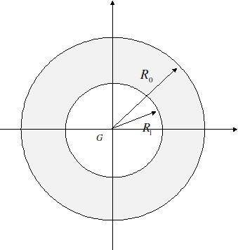
We have the following problem to solve:

\(\Delta \psi =-2\)

\(\psi (r={R}_{0})={\psi }_{0}=0\)

\(\psi (r={R}_{1})={\psi }_{1}\)

\({\int }_{\partial {\Omega }_{1}}\frac{\partial \psi }{\partial n}\text{dl}=2\pi {R}_{0}^{2}\)

The general solution to the problem is spelled \(\psi =\psi (r)\text{=-}\frac{{r}^{2}}{2}+A\text{ln}(r)+B\)

Here, we have \(\frac{\partial \psi }{\partial n}{\mid }_{\partial {\Omega }_{1}}=-\frac{\partial \psi }{\partial r}{e}_{r}\). Hence \(2\pi {R}_{1}^{2}-2\pi A\text{ln}({R}_{1})=2\pi {R}_{1}^{2}\Rightarrow A=0\). On the other hand, we have \(\psi ({R}_{0})=0\Rightarrow B=\frac{{R}_{0}^{2}}{2}\). Finally:

\(\psi (r)\text{=-}\frac{{r}^{2}}{2}+\frac{{R}_{0}^{2}}{2}\).

Now we can calculate \(J=2{\int }_{\Omega }\psi \text{ds}+2{\psi }_{1}A(\partial {\Omega }_{i})\). We have \({\psi }_{1}\text{=}-\frac{{R}_{1}^{2}}{2}+\frac{{R}_{0}^{2}}{2}\) and \(A(\partial {\Omega }_{1})=\psi {R}_{1}^{2}\). All calculations done, we have the classic result: \(J=\frac{\pi }{2}({R}_{0}^{4}-{R}_{1}^{4})\)

Determination of the shear constant of a beam equivalent to a set of parallel beams

Problem position:

Here we explain a method developed in command MACR_CARA_POUTRE to obtain the coefficients \(\mathrm{AY}\) and \(\mathrm{AZ}\) of a beam equivalent to a set of disjoint beams (e.g. columns embedded between two floors). This makes it possible, for example, to produce « skewer » models of buildings, that is to say, condensed into a single beam.

For a single beam, the definition of shear coefficients is based on the energetic method [§2.1.3]: the formulation is based on the complementary energy due to shear in the section.

The shear coefficient is: \(k\text{=}{\frac{\left[{\int }_{s}{\sigma }_{\text{CT}}\text{dS}\right]}{SG{\int }_{s}\frac{1}{G}{\sigma }_{{\text{CT}}^{2}}\text{dS}}}^{2}\)

Note:

This expression is valid in the case of a heterogeneous beam ( \(G\) variable) .

The shear stress distribution in the section, for a single beam, is based on the Jourawski formula, [§2.1.1] which provides the distribution of shear stresses due to shear force in one direction and only the average of shear stresses in the other direction.

Jourawski’s formula is written as:

\({\sigma }_{\text{CT}}=\frac{m(y)}{\mathrm{Ib}(y)}V\) with \(m(y)\text{=}{\int }_{y}^{{y}_{\text{max}}}t\text{}b(t)\text{}\text{dt}\)

The quantity \(m(y)\) represents the static moment for the part of section \(A\) between \(y\) and \({y}_{\mathrm{max}}\)

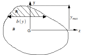
So \(k\) can be written in the form: \(k=\frac{{I}^{2}}{S\text{G}{\int }_{y}^{{y}_{\text{max}}}\frac{{m}^{2}(y)}{{\text{Gb}}^{2}(y)}\text{dy}}\)

The underlying idea is that the section supports normal stresses from Euler’s beam theory, and that we evaluate the sliding force of \(A\) over \(B\).

For a non-connected section, such as the cross-section of a building, Jourawski’s hypothesis cannot be made (except considering that the entire section deforms axially like the same beam at each abscissa \(x\)). It is not possible to know at first glance the distribution of shears or of the normal stresses in each column. The following figure gives an idea of the cross-sectional view of a reactor building:

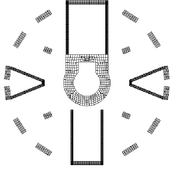
Figure 11 : Section of a reactor building

Simplified expression of shear coefficients

Hypothesis: the posts are embedded in the floors: the building seen from the side can be represented as a set of parallel posts embedded between two floors:

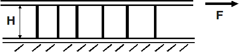
Figure 12 : set of posts between two boards

This particular case is calculated: each column is a beam with a rectangular cross section (the main axes of inertia of the various columns are not collinear). \(H=3\) to \(\mathrm{4m}\).

The beams are embedded at both ends. It is then necessary to find a relationship between an effort \(F\) imposed on the upper floor, and the movement of this floor in the same direction, i.e. calculate the stiffness of this system in this direction.

• For a beam:

The method used is explained for example in [bib].

• Beam embedded at one end and free at the other:

The system is isostatic and elastic. We want to express displacement \(u(H)\) in terms of \(F\) and \(\Gamma\). The Principle of Virtual Work is written as:

\(\begin{array}{}f(H)\mathrm{.}v(H)=\underset{0}{\overset{H}{\int }}{M}^{f}\mathrm{.}\kappa (v)+{V}^{f}\mathrm{.}\gamma (v)\mathrm{dl}\\ \kappa (v)=\frac{M(v)}{\mathrm{E.}I}\\ \gamma (v)=\frac{V(v)}{\mathrm{G.}{S}_{r}}\end{array}\)

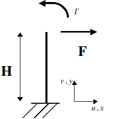
for any virtual \(v\) movement, and for a one-off effort \(f\) in \(y=H\), (here the normal effort is zero). We choose \(f=1\), and we calculate successively the displacements due to an effort \(F\) and to a couple \(\Gamma\) in \(y=H\). Integrating the previous expression, we find that, under the effect of \(F\), the real \(u\) displacement and the rotation equal: \(u(H)=\frac{F\text{.}{H}^{3}}{3E\text{.}I}+\frac{F\text{.}H}{G\text{.}{S}_{r}}=\frac{F\text{.}{H}^{3}}{\text{12}E\text{.}I}(4+\frac{\text{12}\text{EI}}{G\text{.}{H}^{2}{S}_{r}})\) with \({S}_{r}=k\cdot S\) and \(\theta (H)\text{=}-\frac{F\text{.}{H}^{2}}{2E\text{.}I}\)

Under the effect of moment \(\Gamma\), we get:

\({u}_{\Gamma }(H)\text{=}-\frac{\Gamma \text{.}{H}^{2}}{2E\text{.}I}\) \({\theta }_{\Gamma }(H)=\frac{\Gamma \text{.}H}{E\text{.}I}\)

If the beam has a rectangular cross section with a width \(b\) and a thickness \(h\), we get: \({S}_{r}=\text{bhk}=\text{bh}\frac{5}{6}\)

for F imposed: \(u(H)=\frac{F\text{.}{H}^{3}}{E\text{.}{\text{bh}}^{3}}(4+\frac{\text{12}}{5}\frac{{h}^{2}}{{H}^{2}}(1+\nu ))\) \(\theta (H)\text{=-}\frac{6F\text{.}{H}^{2}}{E\text{.}{\text{bh}}^{3}}\) for \(\Gamma\) imposed: \({u}_{\Gamma }(H)\text{=}-\frac{6\Gamma \text{.}{H}^{2}}{E\text{.}{\text{bh}}^{3}}\) \({\theta }_{\Gamma }(H)=\frac{\text{12}\Gamma \text{.}H}{E\text{.}{\text{bh}}^{3}}\)

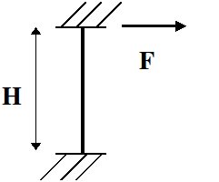
• Beam embedded at both ends: (sliding recess in \(y=H\) )

The system is hyperstatic of degree 1. The displacement \(u(H)\) is expressed as a function of the hyperstatic unknowns \(F\) and \(\Gamma\) using the previous results. Under the effect of \(F\) and \(\Gamma\), the displacement of the real and the rotation (zero because of the embedment) are equal to:

\(\begin{array}{}u(H)=\frac{F\mathrm{.}{H}^{3}}{3\mathrm{E.}I}+\frac{\mathrm{F.}H}{G{S}_{r}}-\frac{\Gamma \mathrm{.}\mathrm{H²}}{2\mathrm{E.}I}=\frac{F\mathrm{.}{H}^{3}}{\mathrm{E.}b{h}^{3}}(4+\frac{12}{5}\frac{\mathrm{h²}}{\mathrm{H²}}(1+\nu ))\\ 0=-\frac{F\mathrm{.}\mathrm{H²}}{2EI}+\frac{\Gamma \mathrm{.}H}{\mathrm{E.}I}=-\frac{6F\mathrm{.}\mathrm{H²}}{E\mathrm{.}bh}+\frac{12\Gamma \mathrm{.}H}{E\mathrm{.}\mathrm{bh²}}\end{array}\)

The resolution of this system makes it possible to obtain u (H) as a function of F:

\(\begin{array}{}u(H)=\frac{F\text{.}{H}^{3}}{\text{12}\text{EI}}(1+\frac{\text{12}\text{EI}}{{\text{GH}}^{2}{S}_{r}})=\frac{F\text{.}{H}^{3}}{E\text{.}{\text{bh}}^{3}}(1+\frac{\text{12}}{5}\frac{{h}^{2}}{{H}^{2}}(1+\nu ))\\ F=(\frac{\text{12}\text{EI}}{{H}^{3}}\frac{1}{(1+\frac{\text{12}\text{EI}}{{\text{GH}}^{2}{S}_{r}})})u(H)=(\frac{E\text{.}{\text{bh}}^{3}}{{H}^{3}}\frac{1}{(1+\frac{\text{12}}{5}\frac{{h}^{2}}{{H}^{2}}(1+\nu ))})u(H)=K\text{.}u(H)\end{array}\)

We also find this result by considering the stiffness matrix of an « exact » 2-node beam element ([bib] or [R3.08.01]). The term above corresponds exactly to the term shear force stiffness alone in the direction x:

\({K}_{\text{xx}}=(\frac{\text{12}\text{EI}}{{H}^{3}}\frac{1}{(1+\Phi )})\Phi =\frac{\text{12}\text{EI}}{{\text{GH}}^{2}{S}_{r}}=\frac{\text{12}\text{EI}}{{\text{GH}}^{2}\text{kS}}\)

Note:

The built-in free situation only differs by one coefficient (4 instead of 1),:

\(u(H)=\frac{F\text{.}{H}^{3}}{E\text{.}{\text{bh}}^{3}}(4+\frac{\text{12}}{5}\frac{{h}^{2}}{{H}^{2}}(1+\nu ))\)

Both options are offered in MACR_CARA_POUTRE:

• both ends are embedded (in reality one is embedded, the other is embedded in a mobile floor: sliding installation)

• the upper end is free (in fact in a swivel connection with the upper floor).

It is therefore possible to propose to express the shear force stiffness of each column in the form:

\(F=(\frac{\text{12}\text{EI}}{{H}^{3}}\frac{1}{(\xi +\frac{\text{12}\text{EI}}{{\text{GH}}^{2}{S}_{r}})})u(H)=K\text{.}u(H)\) with \(\xi =\{\begin{array}{c}1\text{encastré}-\text{encastré}\\ 4\text{encastré}-\text{libre}\end{array}\)

For a set of beams

The method consists in calculating the stiffness of each column in the previous way, and in comparing the stiffness of the whole to that of an equivalent beam embedded between two floors. To do this, we express the overall shear force applied to all the posts (for example in the \(y\) direction):

\({T}_{y}=\sum {T}_{i}={\tilde{K}}_{y}\text{.}{u}_{y}\)

Since each column has any orientation in relation to the global axes, it is first of all necessary to express the \({T}_{i}\) efforts in the global coordinate system:

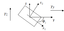
\({x}_{1}\) and \({x}_{2}\) designating the main axes of inertia of the column i, the shear force \({T}_{i}\) in this coordinate system is: \(\begin{array}{}{T}_{y}^{i}={T}_{1}^{i}\text{cos}({\varphi }_{i})+{T}_{2}^{i}\text{sin}({\varphi }_{i})\\ {T}_{z}^{i}\text{=-}{T}_{1}^{i}\text{sin}({\varphi }_{i})+{T}_{2}^{i}\text{cos}({\varphi }_{i})\end{array}\)

In addition, it is assumed that the global displacement \(u\) of all the posts is uniform (with components \({u}_{x}\) and \({u}_{y}\)) and must be collinear to the shear force \(T\). (which is not certain: couplings are possible if there are no particular symmetries). For direction \(y\), this means:

\(\begin{array}{}{u}_{1}^{i}={u}_{y}\text{cos}({\varphi }_{i})\\ {u}_{2}^{i}={u}_{y}\text{sin}({\varphi }_{i})\end{array}\) and \(\begin{array}{}{T}_{1}^{i}={K}_{1}^{i}\text{.}{u}_{1}^{i}\\ {T}_{2}^{i}={K}_{2}^{i}\text{.}{u}_{2}^{i}\end{array}\)

we get:

\(\begin{array}{}{T}_{y}^{i}=({K}_{1}^{i}{\text{cos}}^{2}({\varphi }_{i})+{K}_{2}^{i}{\text{sin}}^{2}({\varphi }_{i})){u}_{y}^{i}\\ {T}_{y}=\sum {T}_{y}^{i}=\sum ({K}_{1}^{i}{\text{cos}}^{2}({\varphi }_{i})+{K}_{2}^{i}{\text{sin}}^{2}({\varphi }_{i})){u}_{y}={\tilde{K}}_{y}{u}_{y}\end{array}\) with \({\tilde{K}}_{y}=\frac{\text{12}\text{EI}}{{H}^{3}}\frac{1}{(\xi +\frac{\text{12}\text{EI}}{{\text{GH}}^{2}{S}_{r}})}\)

similarly in direction \(z\):

\(\begin{array}{}{u}_{1}^{i}\text{=}-{u}_{z}\text{sin}({\varphi }_{i})\\ {u}_{2}^{i}={u}_{z}\text{cos}({\varphi }_{i})\end{array}\) so \({T}_{z}=\sum {T}_{z}^{i}=\sum ({K}_{1}^{i}{\text{sin}}^{2}({\varphi }_{i})+{K}_{2}^{i}{\text{cos}}^{2}({\varphi }_{i})){u}_{z}={\tilde{K}}_{z}{u}_{z}\)

On the other hand, for the equivalent beam, it is assumed that the stiffness under shear force is expressed in the same way as that of each beam:

\({T}_{y}={K}_{{}_{y}}^{\text{eq}}{u}_{y}=\frac{\text{12}{\text{EI}}_{z}^{\text{eq}}}{{H}^{3}(1+{\Phi }_{y})}{u}_{y}\text{avec}{\Phi }_{y}=\frac{\text{12}{\text{EI}}_{z}^{\text{eq}}}{{S}^{\text{eq}}{H}^{2}{\text{Gk}}_{y}^{\text{eq}}}\)

In fact, it should be verified that the energies due to flexure and normal effort are very negligible. The two expressions of shear force lead to the expression of the equivalent shear coefficient: \({k}_{y}^{\text{eq}}=\frac{\text{12}{\text{EI}}_{z}^{\text{eq}}}{{\text{GS}}^{\text{eq}}{H}^{2}(\frac{\text{12}{\text{EI}}_{z}^{\text{eq}}}{{H}^{3}{\tilde{K}}_{y}}-1)}\) and in the direction \(z\): \({k}_{z}^{\text{eq}}=\frac{\text{12}{\text{EI}}_{y}^{\text{eq}}}{{\text{GS}}^{\text{eq}}{H}^{2}(\frac{\text{12}{\text{EI}}_{y}^{\text{eq}}}{{H}^{3}{\tilde{K}}_{z}}-1)}\)

Method used in MACR_CARA_POUTRE

Using the assumptions described above, namely:

• only the stiffness due to the shear force is taken into account in the calculation of the shear coefficients

• the equivalent beam is embedded on both floors

• two calculation hypotheses are to be expected concerning each pole (recessed and swivel and recessed and recessed).

A calculation method can be proposed in MACR_CARA_POUTRE to obtain shear coefficients equivalent to a set of beams with parallel axes, embedded in a floor at one of their ends, and free at the other, or embedded at the other end.

Restrictions on use:

• it is reasonable to place the equivalent beam on the center of gravity of the set of columns, and in the main inertia coordinate system of the set, to avoid parasitic couplings

• it is necessary to ensure the continuity of all the degrees of freedom of the equivalent beam (translation and rotation) with the degrees of freedom of the floors (which models the embedment of the beam in the floor), which requires modeling the floor in shell elements or, if it is meshed in 3D, to connect it using beams or plates.

The calculation method is as follows:

• For each column, perform the usual calculation using geometric characteristics and shear coefficients of the section, in the main inertia coordinate system of each section (already available).

• Always for each section, calculation of the shear stiffness (the user must provide H, distance between floors).

\(\begin{array}{}{K}_{1}^{i}=\frac{\text{12}{\text{EI}}_{2}^{i}}{{H}^{3}(1+{\Phi }_{1})}\text{avec}{\Phi }_{1}=\frac{\text{12}{\text{EI}}_{2}^{i}}{{S}^{i}{H}^{2}{\text{Gk}}_{1}^{i}}\\ {K}_{2}^{i}=\frac{\text{12}{\text{EI}}_{1}^{i}}{{H}^{3}(1+{\Phi }_{2})}\text{avec}{\Phi }_{2}=\frac{\text{12}{\text{EI}}_{1}^{i}}{{S}^{i}{H}^{2}{\text{Gk}}_{2}^{i}}\end{array}\)

• Calculation of the stiffness equivalent to all the beams:

\({\tilde{K}}_{y}=\sum ({K}_{1}^{i}{\text{cos}}^{2}({\varphi }_{i})+{K}_{2}^{i}{\text{sin}}^{2}({\varphi }_{i}))\)

\({\tilde{K}}_{z}=\sum ({K}_{1}^{i}{\text{sin}}^{2}({\varphi }_{i})+{K}_{2}^{i}{\text{cos}}^{2}({\varphi }_{i}))\)

• Calculation of equivalent shear coefficients:

\({k}_{y}^{\text{eq}}=\frac{\text{12}{\text{EI}}_{z}^{\text{eq}}}{{\text{GS}}^{\text{eq}}{H}^{2}(\frac{\text{12}{\text{EI}}_{z}^{\text{eq}}}{{H}^{3}{\tilde{K}}_{y}}-1)}\)

knowing that \({S}^{\mathrm{eq}}\), \({I}_{y}^{\mathrm{eq}}\) and \({I}_{z}^{\mathrm{eq}}\) are already calculated by MACR_CARA_POUTRE.

For the keywords in command MACR_CARA_POUTRE, the user must provide \(H\), with the keyword LONGUEUR, the characteristics (constants) of the material (keyword MATERIAU) and choose the boundary conditions with the keyword LIAISON:

LIAISON: ROTULE or LIAISON: ENCASTREMENT

This calculation is of course only activated if several GROUP_MA are defined by the user (indicating that the section is composed of disjoint subparts).