10. Dynamic problem#
This problem is that of calculating the evolution of a cable structure.
10.1. Iterative time integration algorithm#
The discretized form of [eq] and [eq] complete, which must be satisfied at every node and at every moment is:
\({F}_{\text{int}}(t)-{F}_{\text{iner}}(t)={F}_{\text{ext}}(t)\) [11]
The time integration algorithm is of the Newmark [bib] and [bib] type. Suppose that the state of the cable (fields \(u,\dot{u}\mathrm{et}\ddot{u}\) at the nodes) is known at time \(t\) and that we have just calculated an approximate value of these fields at the nth iteration of time \(t+\Delta t\).
If these values satisfy [eq], except for one tolerance, they are taken as field values at time \(t+\Delta t\).
Otherwise, we are looking for displacement correction \(\Delta {u}^{n+1}\), to which, according to the Newmark algorithm, the speed and acceleration corrections correspond to:
\(\Delta {\dot{u}}^{n+1}=\frac{\gamma }{\beta \Delta t}\Delta {u}^{n+1}\)
and
\(\Delta {\ddot{u}}^{n+1}=\frac{1}{\beta \Delta {t}^{2}}\Delta {u}^{n+1}\)
such as:
\(\left[{K}_{M}^{n}+{K}_{G}^{n}+\frac{1}{\beta \Delta {t}^{2}}M\right]\Delta {u}^{n+1}={F}_{\text{ext}}(t+\Delta t)-{F}_{\text{int}}^{n}(t+\Delta t)+{F}_{\text{iner}}^{n}(t+\Delta t)\)
In cable movement analysis, the Newmark algorithm may be unstable. This is why we use the algorithm called HHT, defined in [bib5, bib7], in which the two Newmark parameters are functions of a third parameter \(\alpha\):
\(\begin{array}{c}\gamma =\frac{1}{2}-\alpha \\ \beta =\frac{{(1-\alpha )}^{2}}{4}\\ \alpha \le 0\end{array}\)
For \(\alpha =0\), the algorithm is that of Newmark, known as the « trapezium rule ». But for \(\alpha\) being slightly negative, in practice: \(\alpha \ge -0.3\), there appears to be numerical amortization that stabilizes the calculation.
Determining the initial acceleration and initializing the fields at the start of a new time step are shown in [bib].
10.2. Comparison of short circuit calculations and tests#
To validate this cable modeling, we compared dynamic calculations by*Code_Aster* to short circuit test results [bib8]. These were carried out at the EDF Electrical Engineering Laboratory on an experimental structure representative of station configurations [Figure]. Three cables stretched between two gantries distant from \(\mathrm{102 }m\) are shorted, in the foreground, by a shunt arranged on insulating columns.
At the other gantry, they are powered by a three-phase current of \(35\mathrm{kA}\) during \(\mathrm{250 }\mathrm{ms}\). The evolution has been recorded:
from the tension of the cables to their anchoring on the gantries, using dynamometers;
the movement of the mid-points of the ranges, identified by signaling spheres, using fast cameras. We see the glass cage of one of these cameras mounted on a gantry, to the left of [Figure].
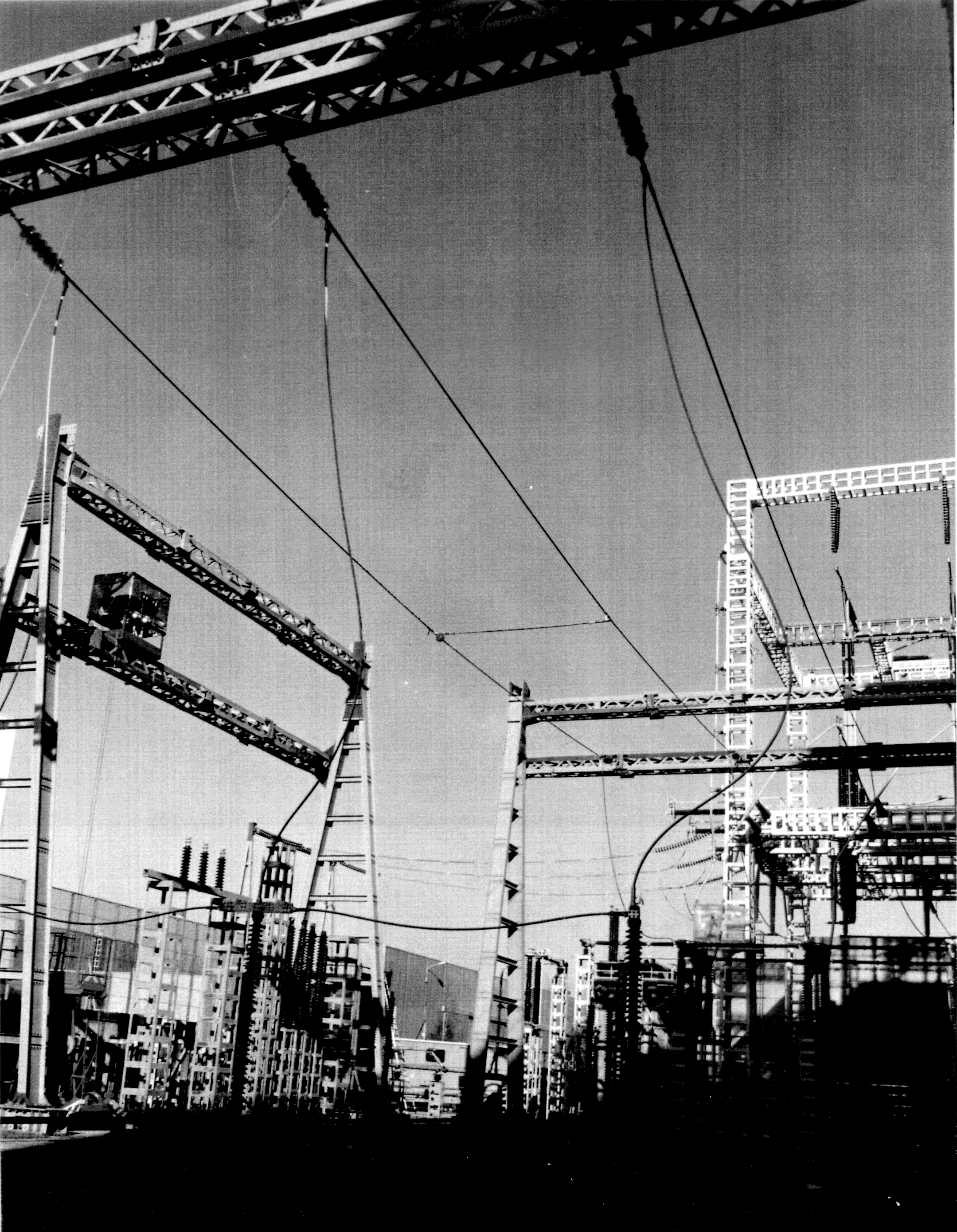
Figure 3: Overview of the short circuit test facility
The [Figure] gives the comparison for an anchoring tension and for the displacement of the middle of a cable.
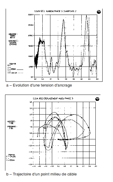
Figure 4: Comparisons of Code_Aster calculations and short circuit tests