12. Bibliography#
[1] J.L. LILIEN: Electromechanical constraints and consequences related to the passage of current intensity in cable structures. Thesis. University of Liège (1983).
[2] J.C. SIMO, L. VU- QUOC: A three-dimensional finite-strain rod model. Part II: computational aspects, Comput. Meth. call. Mech. Engng, Vol. 58, p.79-116 (1986).
[3] A. CARDONA, M. GERADIN: A beam finite element nonlinear theory with finite rotations, Int. Mr Numer. Meth. Engng. Vol. 26, p.2403-2438 (1988).
[4] R.L. WEBSTER: On the static analysis of structures with strong geometric non-linearity. Computers & Structures 11, 137-145 (1980).
[5] N. GREFFET, F. VOLDOIRE, M. AUFAURE: Dynamic nonlinear algorithm. Document R5.05.05.
[6] K.J. BATHE: Finite element procedures in engineering analysis. Prentice-Hall (1982).
[7] H.M. HILBER, T.J.R. HUGHES, R.L., R.L. TAYLOR: Improved numerical dissipation for time integration algorithms in structural dynamics. Earthq. Engng Struct. Dyn. 5, 283-292 (1977).
[8] F. DURAND: Three-phase line range (102m) for THT stations. Test report. EDF (1990).
Document version history
Doc index |
Version Aster |
Author (s) or contributor (s), organization |
Description of changes |
A |
3 |
M. AUFAURE 1 G. DEVESA1 1 EDF /R & D |
Initial text |
B |
9.4 |
J.L. FLEJOU EDF /R &D/ AMA |
The temperature is no longer affected by the AFFE_CHAR_MECA command but by affe_materiau/affe_varc |
C |
12.3 |
F. VOLDOIRE EDF /R &D/ AMA |
Some corrections of form (§ 1, 3, 4…) and references in nonlinear dynamics § 10. |
: Calculation of Laplace forces between conductors Any conductor that a current flows through creates a magnetic field in its vicinity. This magnetic field, acting on the current carried by another conductor, induces on this one a so-called Laplace force.
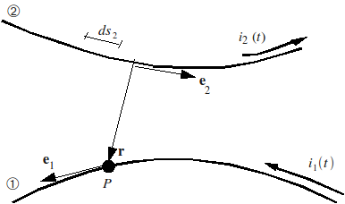
Figure 5: Arrangement of two neighboring conductors
Let’s take a conductor \((1)\) through which the current \({i}_{1}(t)\) [Figure A1-a] flows, located in the vicinity of the conductor \((2)\) through which the current \({i}_{2}(t)\) flows. At the point P of conductor \((1)\), where the unit tangent oriented in the direction of the current is \({e}_{1}\), the linear Laplace force induced by conductor \((2)\) is:
\(f(P)={\text{10}}^{-7}{i}_{1}(t){i}_{2}(t){e}_{1}\times {\int }_{{\Gamma }_{2}}^{}{e}_{2}\times \frac{r}{{r}^{3}}{\mathrm{ds}}_{2}\)
We are only interested in the forces due to very intense short-circuit currents, the Laplace forces under normal conditions being negligible.
\(f(P)\) can obviously be put in the form of the product of a function of time by a function of space.
A1.1 Function of the time of the Laplace forces
This function \(g(t)\), except for one factor, is the product of the intensities in conductors \((1)\) and \((2)\):
\(g(t)=2.{\text{10}}^{-7}{i}_{1}(t){i}_{2}(t)\) [12]
where:
\({i}_{j}(t)=\sqrt{2}{I}_{\text{ej}}\left[\text{cos}(\omega t+{\varphi }_{j})-{e}^{-t/\tau }\text{cos}{\varphi }_{j}\right]\) [13]
with:
\({I}_{\text{ej}}\): |
effective current strength j; |
\(\omega\): |
current pulsation (\(\omega =100\pi\) for a current of 50Hz); |
\({\varphi }_{j}\): |
phase depending on when the short circuit occurs; |
\(\tau\): |
time constant of the short circuit line depending on its electrical characteristics (self, capacitance and resistance). |
Very often, we replace the complete function \(g(t)\) [eq] and [eq] by its mean - which is called the continuous part - by neglecting the terms \(\mathrm{cos}(\omega t+\mathrm{...})\) and \(\mathrm{cos}(2\omega t+\mathrm{...})\). Taking these terms into account would require a very small step of time and the corresponding forces, at \(50\mathrm{Hz}\) and \(\mathrm{100 }\mathrm{Hz}\), have almost no effect on cables whose oscillation frequency is of the order of one Hertz.
So:
\({g}_{\text{continue}}(t)=2{I}_{\mathrm{e1}}{I}_{\mathrm{e2}}\left[\frac{1}{2}\text{cos}({\varphi }_{1}-{\varphi }_{2})+{e}^{-(\frac{t}{{\tau }_{1}}+\frac{t}{{\tau }_{2}})}\text{cos}{\varphi }_{1}\text{cos}{\varphi }_{2}\right]\)
A1.2 Space function
This function is:
\(h(P)=\frac{1}{2}{e}_{1}\times \int {e}_{2}\times \frac{r}{{r}^{3}}{\mathrm{ds}}_{2}\)
The integral is calculated analytically when conductor \({\Gamma }_{2}\) is divided into rectilinear elements. Along with such an element \({M}_{1}{M}_{2}\) [Figure A1.2-a], we have an effect:
\(\begin{array}{}{r}^{3}={({y}^{2}+{r}_{m}^{2})}^{}\\ {e}_{2}\times r={e}_{2}\times {r}_{m}\\ {\mathrm{ds}}_{2}=\text{dy}\end{array}\)
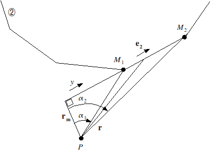
Figure 6: Laplace force induced by a rectilinear conductor element
Like:
\({\int }_{{y}_{1}}^{{y}_{2}}\frac{\text{dy}}{{({y}^{2}+{r}_{m}^{2})}^{}}=\frac{1}{{r}_{m}^{2}}{\left[\frac{y}{{({y}^{2}+{r}_{m}^{2})}^{}}\right]}_{{y}_{1}}^{{y}_{2}}\)
we have:
\(\frac{1}{2}{e}_{1}\times {\int }_{{M}_{1}}^{{M}_{2}}{e}_{2}\times \frac{r}{{r}^{3}}\mathrm{dy}=\frac{1}{2{r}_{m}^{2}}{e}_{1}\times {e}_{2}\times {r}_{m}{\left[\frac{y}{{({y}^{2}+{r}_{m}^{2})}^{}}\right]}_{{y}_{1}}^{{y}_{2}}\)
The hook on the second member is also equal to:
\(\text{sin}{\alpha }_{2}-\text{sin}{\alpha }_{1}\).
A1.3 **Realization in***Code_Aster*
The space function \(h(P)\) defined above is calculated by an elementary routine that evaluates, for each of the elements of the conductor \((1)\), the contribution of all the elements of the conductor \((2)\) that act on it.
This contribution is evaluated at the Gauss points (only 1 for 2-node elements) of the conductor element, \((1)\) by the INTE_ELEC keyword of the AFFE_CHAR_MECA command.
The basic routine has 2 input parameters:
the loading map of the conductor element \((1)\) including the list of the cells of the conductor \((2)\) acting on it;
the name of the geometry, which varies over time, which allows quantities \({r}_{m},\text{sin}{\alpha }_{1},\text{sin}{\alpha }_{2}\) to be evaluated at any moment.
The time function \(g(t)\) is calculated by the operator DEFI_FONC_ELEC which produces a function-like concept.
A1.4 **Use in***Code_Aster*
Definition of the function of time \(g(t)\)
Command |
Factor Key |
Keyword |
Argument |
|
“COMPLET” |
||||
DEFI_FONC_ELEC |
SIGNAL |
or |
||
“CONTINU” |
||||
COUR |
|
|
||
TAU_CC_1 |
|
|||
PHI_CC_1 |
|
|||
INTE_CC_2 |
|
|||
TAU_CC_2 |
|
|||
PHI_CC_2 |
|
|||
INST_CC_INIT |
Short-circuit start time. |
|||
INST_CC_FIN |
Short-circuit end instant. |
Definition of the function of space \(h(P)\)
Command |
Factor Key |
Keyword |
Argument |
AFFE_CHAR_MECA |
MODELE |
Model name. |
|
INTE_ELEC |
|
Name of the group of elements for conductor \((1)\). |
|
GROUP_MA_2 |
Name of the group of elements of the \((2)\) conductor. |
Taking into account Laplace’s strengths
Command |
Factor Key |
Keyword |
Argument |
DYNA_NON_LINE |
|
|
name of \(h(P)\) |
FONC_MULT |
name of \(g(t)\) |
: Calculation of the force exerted by the wind A3.1 Formulation
It is assumed that a wind of speed \(V\) exerts in the vicinity of the point \(P\) of a cable [Figure] an aerodynamic linear force \(f\) having the following characteristics:
\(f\) has the direction and direction of the \({V}_{n}\) wind speed component in the normal plane of the cable.
\(f\) has a modulus that is proportional to the square of that of \({V}_{n}\).
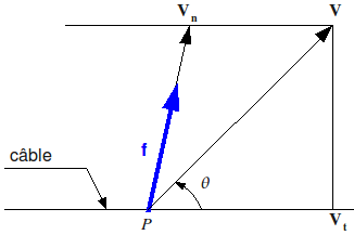
Figure 7: Wind speed in the vicinity of a cable
The rules for calculating lines define the strength of a wind by the pressure \(p\) it exerts on a flat surface normal to its direction. For a cable, normally placed in the direction of the wind, these regulations prescribe to take the linear force as follows: \({f}_{\frac{\pi }{2}}\mathrm{=}p\mathrm{\varnothing }\),
\(\varnothing\) being the diameter of the cable. This is equivalent to considering that the cable offers the wind a flat surface equal to its master torque. An increase in force is thus obtained because the cable, which is cylindrical, has less air resistance than a flat surface.
If wind speed \(V\) makes an angle \(\theta\) with the cable, its component in the plane perpendicular to the cable has the module: \(\parallel {V}_{n}\parallel =\parallel V\parallel \mathrm{.}\mid \text{sin}\theta \mid\).
So the linear force is: \({f}_{\theta }\mathrm{=}p\mathrm{\varnothing }{\text{sin}}^{2}\theta\).
Of course, the linear force exerted by the wind depends on the position of the cable: it is « following ».
A3.2 **Use in***Code_Aster*
Here’s how to introduce wind force in*Code_Aster*. The unit vector with the direction and direction of wind speed has components \({v}_{x},{v}_{y},{v}_{z}\).
Command |
Factor Key |
Keyword |
Argument |
AFFE_CHAR_MECA |
|
|
“VENT” |
FX |
\(p\varnothing {v}_{x}\) |
||
FY |
\(p\varnothing {v}_{y}\) |
||
FZ |
\(p\varnothing {v}_{z}\) |
: Modeling cable installation A cable being laid in a canton (several spans between posts) [Figure] is fixed to one of the stop supports. It rests on pulleys placed at the bottom of the alignment insulators and is retained by a force at the level of the second stop support.
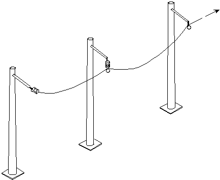
Figure 8: Laying a cable in a two-span township
By playing on this force - or by moving its point of application - we adjust the arrow of one of the ranges, the one that is most subject to environmental constraints. Then the pulleys are removed and the cable is fixed to the insulators: the length of the cable in the various ranges is then fixed. It is on this configuration that additional components are possibly mounted: spacers, equipment descents, point masses,… to give the canton its final shape.
This modeling is described in the reference documentation for elements CABLE_POULIE [R3.08.05].