2. Benchmark solution#
2.1. Calculation method used for the reference solution#
Analytical solution was determined by F. Voldoire (EDF R&D/AMA):
Axisymmetric case ( \(\mathrm{2D}\) )
Move fields \(u={U}_{r}(r){e}_{r}\) (blocked in \(z\))
Deformation field: \(\varepsilon (u)=(\begin{array}{ccc}{u}_{r}\text{'}& 0& 0\\ 0& 0& 0\\ 0& 0& \frac{{u}_{r}}{r}\end{array})\) according to \((\begin{array}{c}r\\ z\\ \theta \end{array})\)
Constraint fields: \(\sigma (u)={\sigma }_{l}(\begin{array}{ccc}0& 0& 0\\ 0& 1& 0\\ 0& 0& 0\end{array})(\mathrm{cf.}\mathrm{conditions}\mathrm{aux}\mathrm{limites})\) according to \((\begin{array}{c}r\\ z\\ \theta \end{array})\)
Parallelepipedic case
Move fields \(u={U}_{x}(x){e}_{x}+{U}_{y}(y){e}_{y}\) (blocked in \(z\))
Deformation field: \(\varepsilon (u)=(\begin{array}{ccc}{u}_{x}\text{'}& 0& 0\\ 0& 0& 0\\ 0& 0& {u}_{y}\text{'}\end{array})\) according to \((\begin{array}{c}x\\ z\\ y\end{array})\)
Constraint fields: \(\sigma (u)=\sigma (\begin{array}{ccc}0& 0& 0\\ 0& 1& 0\\ 0& 0& 0\end{array})(\mathrm{cf.}\mathrm{conditions}\mathrm{aux}\mathrm{limites})\) according to \((\begin{array}{c}x\\ z\\ y\end{array})\)
The case can be studied under plane constraints and in \(\mathrm{3D}\).
\(2\nu =\frac{E}{(1+\nu )}\) \(K=\frac{E}{(1-2\nu )}\)
The law of behavior can be written (scalar internal variable \(p\)):
\(\varepsilon =\frac{1}{\mathrm{9K}}\mathrm{tr}\sigma \mathrm{Id}+\frac{1}{2\mu }{\sigma }^{D}+{\varepsilon }^{P}+\alpha (T–{T}^{0})\mathrm{Id}\)
with: \({\sigma }^{D}=\sigma –\frac{1}{3}\mathrm{tr}(\sigma )\mathrm{Id}\) (constraint deviator)
\({\dot{\sigma }}^{P}=\frac{3}{2}\dot{p}\frac{{\sigma }^{D}}{∥{\sigma }_{\mathrm{éq}}∥}\text{et}∥{\sigma }_{\mathrm{éq}}∥=\sqrt{\frac{3}{2}{\sigma }^{D}\mathrm{.}{\sigma }^{D}}\)
\(\dot{p}=0\) if \(f(\sigma ,p)=∥{\sigma }_{\mathrm{éq}}∥–R(p)<0\)
\(\dot{p}\ge 0\) if \(f(\sigma ,p)=0\)
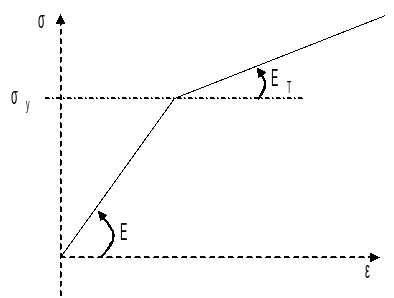
\(R(p)\) refers to the work hardening function: \(R(p)={\sigma }_{y}+\frac{{\mathrm{EE}}_{T}}{E-{E}_{T}}p\)
The \(\dot{p}\) rate can be expressed, when \(f(\sigma ,p)=0\). Indeed, from \(\dot{p}f\) that is identical to zero, we draw: \(\dot{p}\dot{f}+\ddot{p}f=0\)
So, when we are on the criterion, necessarily \(\dot{f}=0\). That is to say:
\(\frac{3}{2}\frac{{\sigma }^{D}\mathrm{.}{\dot{\sigma }}^{D}}{∥{\sigma }_{\mathit{éq}}∥}–\frac{\mathrm{\partial }R}{\mathrm{\partial }T}\mathrm{.}\dot{T}–\frac{\mathrm{\partial }R}{\mathrm{\partial }p}\dot{p}\mathrm{=}0\)
\(\frac{3}{2}\frac{{\sigma }^{D}\mathrm{.}{\dot{\sigma }}^{D}}{∥{\sigma }_{\mathit{éq}}∥}+{\sigma }_{y}^{o}s\dot{T}\mathrm{-}\frac{{\mathit{EE}}_{T}}{E\mathrm{-}{E}_{T}}\dot{p}\mathrm{=}0\)
From where:
\(\dot{p}=\frac{E-{E}_{T}}{{\mathrm{EE}}_{T}}(\frac{3}{2}\frac{{\sigma }^{D}{\dot{\sigma }}^{D}}{∥{\sigma }_{\mathrm{éq}}∥}+{\sigma }_{y}^{o}\mathrm{.}s\mathrm{.}\dot{T})\) if \(\dot{p}\ge 0\), for \(∥{\sigma }_{\mathrm{éq}}∥=R(p)\)
Since the stress field is uniaxial, we have:
\({\sigma }^{D}=\frac{{\sigma }_{L}}{3}(\begin{array}{ccc}-1& 0& 0\\ 0& 2& 0\\ 0& 0& -1\end{array})\)
So:
\(∥{\sigma }_{\mathrm{éq}}∥=∣{\sigma }_{L}∣\)
and:
\({\dot{\varepsilon }}^{P}=\frac{\dot{p}}{2}\mathrm{.}\mathrm{sgn}({\sigma }_{L})\mathrm{.}(\begin{array}{ccc}-1& 0& 0\\ 0& 2& 0\\ 0& 0& -1\end{array})\)
The behavioral relationship leads to:
\(\{\begin{array}{c}\dot{{\varepsilon }_{\mathrm{rr}}}=\dot{{\varepsilon }_{\theta \theta }}=\frac{-\nu }{E}\dot{{\sigma }_{L}}-\frac{\dot{p}}{2}\mathrm{sgn}({\sigma }_{L})+\alpha \dot{T}(={\dot{\varepsilon }}_{\mathrm{xx}}={\dot{\varepsilon }}_{\mathrm{yy}}\text{pour le cas du parallélépipède})\\ \dot{{\varepsilon }_{\mathrm{rr}}}=\dot{{\varepsilon }_{\theta \theta }}=\frac{-\nu }{E}\dot{{\sigma }_{L}}-\frac{\dot{p}}{2}\mathrm{sgn}({\sigma }_{L})+\alpha \dot{T}\end{array}\)
From where:
\(\{\begin{array}{c}\dot{{\varepsilon }_{\mathrm{rr}}}=\dot{{\varepsilon }_{\theta \theta }}=\frac{-3}{2}\alpha \dot{T}+\frac{1-2\nu }{2E}\dot{{\sigma }_{L}}\\ \dot{p}=\mathrm{sgn}({\sigma }_{L})(-\alpha \dot{T}-\frac{\dot{{\sigma }_{L}}}{E})=0\text{si}∣{\sigma }_{L}∣<R(p)\\ \dot{p}=\mathrm{Max}[0,\frac{E-{E}_{T}}{{\mathrm{EE}}_{T}}(\frac{3}{2}\frac{{\sigma }^{D}\dot{{\sigma }^{D}}}{∥{\sigma }_{\mathrm{éq}}∥}+{\sigma }_{y}^{o}\mathrm{.}s\mathrm{.}\dot{T})]\text{sinon}\end{array}\)
That is to say, in case \(∣{\sigma }_{L}∣=R(p)\) (criterion met):
\(\dot{p}=\mathrm{max}\left[0,\frac{E-{E}_{T}}{{\mathrm{EE}}_{T}}(\frac{3}{2}\frac{{\sigma }^{D}\mathrm{.}{\dot{\sigma }}^{D}}{∥{\sigma }_{\mathrm{éq}}∥}+{\sigma }_{y}^{o}\mathrm{.}s\mathrm{.}\dot{T})\right]\)
2.1.1. Elastic phase#
At the start of thermal loading, \(∣{\sigma }_{L}∣\) being less than \({\sigma }_{y}\), \(\dot{p}\) is zero.
From where: \(\dot{{\sigma }_{L}}=-E\alpha \dot{T};\dot{{\varepsilon }_{\mathrm{rr}}}=\dot{{\varepsilon }_{\theta \theta }}=\alpha \dot{T}(1+\nu )\)
So: \(\{\begin{array}{c}{\sigma }_{L}=-E\alpha \theta t\\ {\varepsilon }_{\mathrm{rr}}={\varepsilon }_{\theta \theta }=\alpha \theta (1+\nu )t\end{array}\) (compression \({\sigma }_{L}<0\))
This corresponds to the reference solution for the orthotropic elasticity test
Validity of the elastic solution
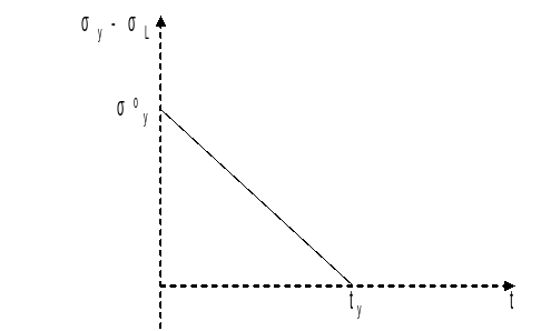
The criterion is: \(∣{\sigma }_{L}(t)∣-{\sigma }_{y}(t)=E=\theta t-{\sigma }_{y}^{o}(1-s\theta t)\le 0\)
The criterion is not met for \(t=[\mathrm{0,}{t}_{y}]\), with: \({t}_{y}=\frac{{\sigma }_{y}^{o}}{\theta (E\alpha +{\sigma }_{y}^{o}s)}\)
At the moment \({t}_{y}\): \({\sigma }_{L}({t}_{y})=\frac{-E\alpha {\sigma }_{y}^{o}}{E\alpha +{\sigma }_{y}^{o}s}\)
The deformation energy density is: :math:`w({t}_{y})=\frac{-1}{2}E{(\alpha \theta )}^{2}`

In the parallelepiped case we have: :math:`w({t}_{y})=\frac{-1}{2}E{(\alpha \theta )}^{2.}({x}_{B}-{x}_{A})H`

In the axisymmetric case we have: :math:`w({t}_{y})=\frac{-1}{2}E{(\alpha \theta )}^{2}\mathrm{.}\frac{({r}_{B}^{2}-{r}_{A}^{2})}{2}H` (for 1 radian)
2.1.2. Elastoplastic phase#
\(t\ge {t}_{y}\). We are on the criteria. So:
\(\dot{p}=\mathrm{max}\left[0,\frac{E-{E}_{T}}{{\mathrm{EE}}_{T}}(\dot{{\sigma }_{L}}\mathrm{sgn}({\sigma }_{L})+{\sigma }_{y}^{o}\mathrm{.}s\mathrm{.}\dot{T})\right]\)
Assuming that you are « in charge » \(\dot{p}\ge 0\), then you eliminate \(\dot{p}\) to have:
\(\dot{{\sigma }_{L}}=-{E}_{T}\mathrm{.}\dot{T}(\alpha +\mathrm{sgn}({\sigma }_{L})\mathrm{.}\frac{E-{E}_{T}}{{\mathrm{EE}}_{T}}{\sigma }_{y}^{o}\mathrm{.}s)\)
then:
\(\dot{p}=\frac{E-{E}_{T}}{E}\dot{T}(-\alpha \mathrm{sgn}({\sigma }_{L})+\frac{{\sigma }_{y}^{o}\mathrm{.}s}{E})\)
\(t={t}_{y}\), \({\sigma }_{L}=-E\alpha \theta {t}_{y}<0\); we then integrate these expressions for \(t\ge {t}_{y}(\dot{T}=\theta )\):
\(\{\begin{array}{c}{\sigma }_{L}(t)=-{E}_{T}\mathrm{.}\theta (t-{t}_{y})[\alpha -\frac{E-{E}_{T}}{{\mathrm{EE}}_{T}}s{\sigma }_{y}^{o}]-{\sigma }_{L}(t-y)\\ p(t)=\frac{{\sigma }_{y}^{o}(E-{E}_{T})}{{E}^{2}}(\frac{t}{{t}_{y}}-1)\end{array}\)
Or, after rearrangement, \(t\ge {t}_{y}\):
\(\mathrm{\{}\begin{array}{c}{\sigma }_{L}(t)\mathrm{=}{\sigma }_{y}^{o}(s\theta t\mathrm{-}1+\frac{{E}_{T}}{E}(1\mathrm{-}\frac{t}{{t}_{y}}))\\ p(t)\mathrm{=}\frac{{\sigma }_{y}^{o}(E\mathrm{-}{E}_{T})}{{E}^{2}}(\frac{t}{{t}_{y}}\mathrm{-}1)\end{array}\)
Validity of this elastoplastic solution
You have to make sure that \({\sigma }_{L}(t)\) stays negative. Knowing that \(s\theta t<1\), and \(t>{t}_{y}\), the previous result confirms that \({\sigma }_{L}(t)<0\). Finally, we note that:
\(\mathrm{sgn}({\sigma }_{L})\frac{1-2\nu }{2}\dot{p}+\dot{{\varepsilon }_{\mathrm{rr}}}=\alpha (1+\nu )\dot{T}\)
from where, since \({\sigma }_{L}(t)<0\):
\({\varepsilon }_{\mathrm{rr}}(t)={\varepsilon }_{\theta \theta }(t)=\alpha \theta (1+\nu )t+\frac{1-2\nu }{2}p(t),\forall t\in \left[{t}_{y},{t}_{\mathrm{fin}}\right]\)
2.1.3. Special case of H and I models#
The thermal deformation is replaced by a given anelastic deformation. Like \(s=0\),
\({\sigma }_{L}=-E\alpha \theta\) \({\varepsilon }_{\mathrm{xx}}={\varepsilon }_{\mathrm{zz}}=\alpha \theta (1+\nu )t\)
The solution remains elastic as long as \(t<{t}_{y}=\frac{{\sigma }_{0}}{\theta E\alpha }=200s\)
2.2. Benchmark results#
\({\varepsilon }_{\mathrm{rr}}\) Or \({\varepsilon }_{\mathrm{xx}}\), \({\sigma }_{\mathrm{zz}}\), and \(p\) in \({t}_{y}\) and beyond:
Elastic phase: for \(t<{t}_{y}\):
\({\sigma }_{L}=-E\alpha \theta t\) \({\varepsilon }_{\mathrm{rr}}={\varepsilon }_{\theta \theta }=\alpha \theta (1+\nu )t\) in axisymmetric
\({\varepsilon }_{\mathrm{xx}}=\alpha \theta (1+\nu )t\) in plane constraints
The elastic limit is reached in \({t}_{y}=\frac{{\sigma }_{0}}{\theta (E\alpha +{\sigma }_{0}s)}=66.666s\) from where \({\sigma }_{L}({t}_{y})=\frac{\sigma }{(1+{\sigma }_{0}\frac{s}{E\alpha })}\)
Elastoplastic phase: for \(t\ge {t}_{y}\)
\({\sigma }_{L}(t)={\sigma }_{0}(s\theta t-1+\frac{{E}_{t}}{E}(1-\frac{t}{{t}_{y}}))\)
\(p(t)=\frac{{\sigma }_{0}(E-{E}_{T})}{{E}^{2}}(\frac{t}{{t}_{y}}-1)\)
\({\varepsilon }_{\mathrm{rr}}={\varepsilon }_{\theta \theta }=\alpha \theta (1+\nu )t+\frac{1-2\nu }{2}p(t)\) in axisymmetric
or \({\varepsilon }_{\mathrm{xx}}={\varepsilon }_{\theta \theta }=\alpha \theta (1+\nu )t+\frac{1-2\nu }{2}p(t)\) in plane constraints
From where:
elastic phase
\(\begin{array}{c}\{\begin{array}{c}{t}_{y}=66.666s\\ {\sigma }_{L}({t}_{y})=-133.333\mathrm{MPa}\end{array}\\ {\varepsilon }_{\mathrm{rr}}({t}_{y})={\varepsilon }_{\theta \theta }({t}_{y})=0.86666{E}^{-3}\end{array}\}\text{phase élastique}\)
\(W=4.44410-3\mathrm{MPa}\)
\(W=0.17778{\mathrm{MPa.mm}}^{2}\) (PLAN or 3D)
\(W=0.26666{\mathrm{Mpa.mm}}^{3}\mathrm{.}\mathrm{rad}-1\) (axi)
Then elastoplastic phase:
\(àt=80s\): \(\sigma (80)=-\mathrm{100.0MPa}\)
\(p(80)=0.300{E}^{-3}\)
\({\varepsilon }_{\mathrm{rr}}(80)={\varepsilon }_{\theta \theta }(80)=1.1{E}^{-3}\)
to \(t\mathrm{=}90s\): \(\sigma (90)=-\mathrm{75.0MPa}\)
\(p(90)=0.525{E}^{-3}\)
\({\varepsilon }_{\mathrm{rr}}(90)={\varepsilon }_{\theta \theta }(90)=1.275{E}^{-3}\)
2.2.1. Special case of H and I models#
To \(t\mathrm{=}66.67s\) \({\sigma }_{L}(66.67)=-133.33\mathrm{MPa}\)
\({\varepsilon }_{\mathrm{xx}}(66.67)={\varepsilon }_{\mathrm{zz}}(66.67)=8.667{E}^{-4}\)
To \(t\mathrm{=}80s\) \({\sigma }_{L}(80)=-160\mathrm{MPa}\)
\({\varepsilon }_{\mathrm{xx}}(80)={\varepsilon }_{\mathrm{zz}}(80)=8.667{E}^{-4}\)
To \(t\mathrm{=}90s\) \({\sigma }_{L}(90)=-180\mathrm{MPa}\)
\({\varepsilon }_{\mathrm{xx}}(90)={\varepsilon }_{\mathrm{zz}}(90)=8.667{E}^{-4}\)
2.3. Uncertainty about the solution#
Analytical solution.