4. B modeling#
4.1. Characteristics of modeling#
This modeling corresponds to the corrected version of the TP. She implements all the proposed calculations, commenting on the results obtained.
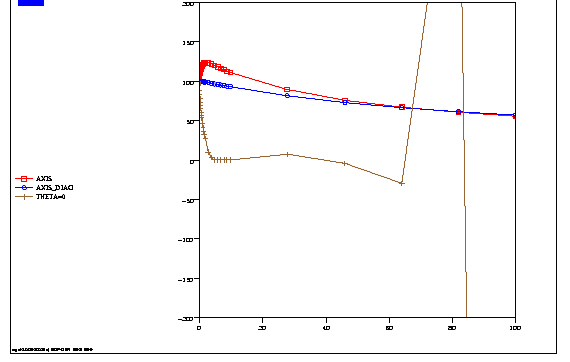
Figure 5.1-a
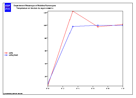
Figure 5.1-b
4.1.1. Thermal calculation#
To improve the results of modeling A, and therefore to compensate for these exceeds the maximum temperature (cf. [R3.06.07]), several solutions are possible:
we can increase the time step, which is not always compatible with a good understanding of the rapidity of the transitory (as in the present case),
or else refine the mesh, which is a good solution, but costly in terms of calculation time,
we can finally use the diagonalization of thermal mass matrices, that is to say here modeling AXIS_DIAG. The curves marked with circles in figures [Figure 5.1-a] and [Figure 5.1-b] above are then obtained. The temperature always stays below \(100°C\). It is the simplest solution.
If we try to use an explicit diagram (\(\mathit{THETA}\mathrm{=}0\)), we see a clear instability appear for large time steps (curve with cross marker in figure [Figure 5.1-a] above).
In conclusion, for thermal calculation, it is necessary to use a \(\mathit{THETA}\) greater than or equal to 0.5, to have a stable pattern regardless of the time step. In addition, it is necessary to use a time step that is small enough to understand the transient, but not too small to avoid oscillations. If they appear, you must either refine the mesh, or use modeling AXIS_DIAG, (or PLAN_DIAG, or 3D_DIAG).
4.1.2. Thermoelastic calculation in free expansion#
The calculation is carried out with MECA_STATIQUE, using thermal expansion as the sole load. With the boundary conditions of the unrestrained case: zero displacement following \(\mathit{Oy}\) along side \(\mathit{AB}\).
For mechanical calculation, it will suffice to calculate at the moments \(t\mathrm{=}\mathrm{0s}\), and \(t\mathrm{=}\mathrm{11s}\) for example.
The constraints at time \(t\mathrm{=}\mathrm{0s}\) are zero, because the temperature field is uniform (\(T\mathrm{=}200°C\)) and remains compatible. On the other hand, the deformations obtained are not zero since the reference temperature is equal to \(200°C\).
At \(t\mathrm{=}\mathrm{11s}\), or any other positive mechanical moment, we see the appearance of so-called thermal compatibility constraints. In fact, the temperature field is no longer uniform but varies according to \(r\). This produces incompatible deformations, which therefore generate stresses, even for an unrestrained cylinder. This situation occurs even for a temperature field that is linear with respect to the radius. On the other hand (see explanation) a temperature field that is linear with respect to the global coordinates does not produce a stress for an unrestrained structure.
4.1.3. Thermoelastic calculation with clamping#
The calculation with MECA_STATIQUE of the BRI case demonstrates the contribution of the clamping on the stresses (\(\mathit{SIYY}\) in particular): at the time \(t\mathrm{=}\mathrm{0s}\), the reference temperature being equal to \(0°C\), the uniform temperature field causes a uniform stress state \(\mathit{SIYY}\) of \(\mathrm{200MPa}\), and at \(t\mathrm{=}\mathrm{11s}\), the stress state is different from the unrestrained case.
This modeling is correct, but is limited to linear behaviors.
4.1.4. Thermoplastic calculation with clamping#
We want to perform the same calculation as before, but this time with STAT_NON_LINE, with COMPORTEMENT =_F (RELATION =” ELAS “), so as not to complicate the problem (another behavior would lead to the same observations). The list of moments provided to STAT_NON_LINEest: \(t\mathrm{=}\mathrm{0s}\) and \(t\mathrm{=}\mathrm{11s}\).
Since an incremental calculation is made, the instant 0 is considered to be the initial moment. It is therefore not calculated, and at the next moment (\(t\mathrm{=}\mathrm{11s}\)), the solution due to the increase in load (thermal here) between \(\mathrm{0s}\) and \(\mathrm{11s}\) is calculated. We then see that the solution obtained (displacements, constraints) is different from the calculation with MECA_STATIQUE. This is logical and consistent with the definition of incremental computation, but it is a trap for use. Remember: implicitly, STAT_NON_LINEen incremental assumes that at the initial moment, the structure is unconstrained, not deformed. This means that the temperature field must be uniform and equal to the reference temperature.
That’s not the case here: at \(t\mathrm{=}\mathrm{0s}\), \(\mathit{TREF}\mathrm{=}0°C\), and \(T\mathrm{=}200°C\). By not calculating this thermal expansion, we assume here that at \(t\mathrm{=}\mathrm{0s}\), there is no deformation, and no stress.
4.1.5. Thermoplastic calculation with clamping and addition of initial conditions#
We modify the list of moments: we add a preliminary moment \(t\mathrm{=}–\mathrm{1s}\) for example. At this moment, a uniform temperature field is defined, equal to the reference temperature. For this purpose, the CREA_CHAMP and then CREA_RESU commands are used to enrich the thermal result data structure with this uniform field. The mechanical calculation is then performed, by providing the list of moments: \(t\mathrm{=}–\mathrm{1s}\), \(t\mathrm{=}\mathrm{0s}\), and \(t\mathrm{=}\mathrm{11s}\)
We then see that the instant \(t=\mathrm{0s}\) is well calculated, and that the constraints are identical to the case calculated with MECA_STATIQUE.
4.2. Characteristics of the mesh#
Same mesh as for modeling A.
4.3. Tested quantities and values#
Modeling AXIS_DIAG
Temperature |
instant |
Identification |
Reference |
Aster |
% difference |
maximum |
4 |
Temp max |
100 |
100 |
0 |