2. Benchmark solution

2.1. Calculation method used for the reference solution

To reduce the time required to set up thermal calculations in the linear domain, a new methodology is proposed.

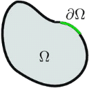
A \(\Omega\) structure is considered. A thermal shock is imposed on a part of the structure \(\partial \Omega\). An example is shown in the following figure.

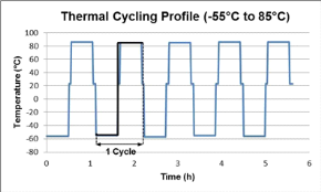
Thermal shock is defined as a significant and instantaneous temperature increment. Figure 2 shows an example of several consecutive thermal shocks.

Fourrier’s law describing heat exchanges applied to this structure subjected to thermal shock can be written in this form:

\(T(x,t)=\{\begin{array}{c}T(x,{t}_{0})\text{pour t <}{t}_{c}\\ T(x,{t}_{0})+\underset{{t}_{c}}{\overset{t}{\int }}a\frac{{\partial }^{2}T(x,t)}{\partial {x}^{2}}\mathit{dt}\text{pour t}\ge \text{}{t}_{c}\end{array}\)

Where \(T(x,{t}_{0})\) is the initial state of the structure, known, and \({t}_{c}\) the instant of the thermal shock. For various thermal shocks, it is therefore necessary to solve this problem and thus obtain, for each of the shocks, solution \(T(x,t)\).

2.1.1. Case of unit shock

If a unit shock \(\mathrm{\Delta }{T}_{U}\) (\(\mathrm{\Delta }T=1\) degree shock) is imposed on \(\partial \Omega\) at time \(t={t}_{c}\), the problem is written as:

\({T}_{U}(x,t)=\{\begin{array}{c}{T}_{U}(x,{t}_{0})\text{pour t <}{t}_{c}\\ {T}_{U}(x,{t}_{0})+\underset{{t}_{c}}{\overset{t}{\int }}a\frac{{\partial }^{2}{T}_{U}(x,t)}{\partial {x}^{2}}\mathit{dt}\text{pour t}\ge \text{}{t}_{c}\end{array}\)

With \({T}_{U}(x,{t}_{0})\) the initial state of the structure before the unity shock. The solution to this problem can be determined numerically using the finite element method, in particular the Code_Aster operator THER_LINEAIRE if the material parameters are independent of temperature. Once the problem is resolved, solution \({T}_{U}(x,t)\) is known.

As we are only interested in the temperature differential, a simplified notation is proposed:

\(\stackrel{̃}{{T}_{U}}(x,t)={T}_{U}(x,t)-{T}_{U}(x,{t}_{0})\)

So we have

\(\stackrel{̃}{{T}_{U}}(x,t)=\{\begin{array}{c}0\text{pour t <}{t}_{c}\\ \underset{{t}_{c}}{\overset{t}{\int }}a\frac{{\partial }^{2}\stackrel{̃}{{T}_{U}}(x,t)}{\partial {x}^{2}}\mathit{dt}\text{pour t}\ge \text{}{t}_{c}\end{array}\)

2.1.2. Case of any shock

A thermal shock, still on \(\partial \Omega\), but of any intensity \(\beta\) is this time imposed. This problem is written in the form:

\({T}_{\beta }(x,t)=\{\begin{array}{c}{T}_{\beta }(x,{T}_{0})\text{pour t <}{t}_{c}\\ {T}_{\beta }(x,{T}_{0})+\underset{{t}_{c}}{\overset{t}{\int }}a\frac{{\partial }^{2}{T}_{\beta }(x,t)}{\partial {x}^{2}}\mathit{dt}\text{pour t}\ge \text{}{t}_{c}\end{array}\)

With \({T}_{\beta }(x,{t}_{0})\) the initial state of the structure before the thermal shock. Using the simplified notation, we get:

\(\stackrel{̃}{{T}_{\beta }}(x,t)=\{\begin{array}{c}0\text{pour t <}{t}_{c}\\ \underset{{t}_{c}}{\overset{t}{\int }}a\frac{{\partial }^{2}{T}_{\beta }(x,t)}{\partial {x}^{2}}\mathit{dt}\text{pour t}\ge \text{}{t}_{c}\end{array}\)

Compared to the previous unit problem, only the intensity of thermal loading has been changed: \(\Delta T=\beta \Delta {T}_{U}\). Indeed, the shock is still on \(\partial \Omega\), it is simply amplified by the scalar \(\beta\). Therefore:

This last equation is only valid for a linear thermal problem and therefore \(\beta\) independent of position. The solution for any thermal shock is therefore:

\(\stackrel{̃}{{T}_{\beta }}(x,t)=\{\begin{array}{c}0\text{pour t <}{t}_{c}\\ \underset{{t}_{c}}{\overset{t}{\int }}a\beta \frac{{\partial }^{2}\stackrel{̃}{{T}_{U}}(x,t)}{\partial {x}^{2}}\mathit{dt}\text{pour t >}{t}_{c}\end{array}\)

In addition, considering that the scalar \(\beta\) is independent of time, which is consistent with a thermal shock, we have:

\(\underset{{t}_{c}}{\overset{t}{\int }}a\beta \frac{{\partial }^{2}\stackrel{̃}{{T}_{U}}(x,t)}{\partial {x}^{2}}\mathit{dt}=\beta \underset{{t}_{c}}{\overset{t}{\int }}a\frac{{\partial }^{2}\stackrel{̃}{{T}_{U}}(x,t)}{\partial {x}^{2}}\mathit{dt}\)

The integral present in this problem equation is in reality the solution obtained previously for the unit shock:

\(\underset{{t}_{c}}{\overset{t}{\int }}a\frac{{\partial }^{2}\stackrel{̃}{{T}_{U}}(x,t)}{\partial {x}^{2}}\mathit{dt}=\stackrel{̃}{{T}_{U}}(x,t)\text{}\mathit{pour}t\ge {t}_{c}\)

The solution to the problem of heat shock of any kind on \(\partial \Omega\) solution obtained for the unit heat shock:

\(\stackrel{̃}{{T}_{\beta }}(x,t)=\beta \mathrm{.}\stackrel{̃}{{T}_{U}}(x,t)\)

It is considered here that the unitary thermal shock takes place at the same instant as the thermal shock \(\Delta {t}_{c}\). If the shock occurs at another moment, simply postpone the solution:

\(\stackrel{̃}{{T}_{\beta }}(x,t)=\beta \mathrm{.}\stackrel{̃}{{T}_{U}}(x,t-({t}_{c}-{t}_{\mathit{c2}}))\)

Where \({t}_{\mathit{c2}}\) is the moment of unity shock. Therefore, by choosing the unit shock so that \({t}_{\mathit{c2}}\) is at time \(t=\mathrm{0s}\), the solution becomes:

\(\stackrel{̃}{{T}_{\beta }}(x,t)=\beta \mathrm{.}\stackrel{̃}{{T}_{U}}(x,t-{t}_{c})\)

It is therefore possible to determine the temperature field of the structure by proceeding as follows:

• Define a uniform initial temperature field on the structure \({T}_{\beta }(x,{t}_{0})\)

• Set up a thermal analysis of a unit shock at time \(t=\mathrm{0s}\) on the structure and obtain the solution of the unit problem and determine \(\stackrel{̃}{{T}_{U}}(x,t)\). It may be a good idea to set an initial temperature of zero so that \(\stackrel{̃}{{T}_{U}}(x,t)={T}_{U}(x,t)\).

• Calculate the solution (in space and time) from a linear combination of the initial situation \(T(x,{t}_{0})\), the intensity of the shock \(\beta\) as well as the solution of the unit shock problem \(\stackrel{̃}{{T}_{U}}(x,t)\).

2.2. Benchmark results

2.2.1. Thermal analyses

The thermal behavior is axisymmetric. Several points across the thickness and two moments are chosen to test the temperature response. The reference results were obtained by Code_Aster and with a linear axisymmetric mesh that is four times finer. The geometric coordinates of the reference points are as follows:

Points	Radius (m)
Intrados	0.018
A	0.0185
B	0.019
C	0.020
D	0.022
Extrados	0.024

To find these reference results, simply change the value of the « Temp_Choc » variable in the test case command file when performing the unit calculations for each of the two models and to read the refined mesh as input.