2. Benchmark solution#
2.1. Modeling A#
2.1.1. Benchmark results#
For the following displacement \(x\), it is given by the « normal » part of the discretes in parallel, which gives:
\({F}_{x}={K}_{\mathit{el}}{u}_{x}+{K}_{n}({u}_{x}+{\mathit{DIST}}_{1})\) if \({u}_{x}<-{\mathit{DIST}}_{1}\),
\({F}_{x}={K}_{\mathit{el}}{u}_{x}\) otherwise.
We get:
Time |
\({u}_{x}\) |
0.5 |
-0.5 |
1.0 |
-0.75 |
2.0 |
-0.75 |
Table 2.1.1-a: Reference Solution
For the following displacement y, it is given by the « tangential » part of the discretes in parallel, which gives:
\(\begin{array}{c}{F}_{y}={k}_{t}\left({u}_{y}-{\delta }_{y}^{0}\right)+{k}_{\mathit{el}}{u}_{y}\\ \delta ={\delta }^{0}\end{array}\) if \(∣{k}_{t}∣\left({u}_{y}-{\delta }^{0}\right)\le \mu ∣{F}_{x}∣\),
\(\begin{array}{c}{F}_{y}=\mu ∣{F}_{x}∣\mathit{sgn}\left({u}_{y}-{\delta }^{0}\right)+{k}_{\mathit{el}}{u}_{y}\\ \delta =u-\mathit{sgn}({u}_{y}-{\delta }^{0})\mu {K}_{n}({u}_{x}+{\mathit{DIST}}_{1})/{K}_{t}\end{array}\) otherwise.
We noted the « sign » function \(\mathit{sgn}\).
We get:
Time |
\({u}_{y}\) |
1.05 |
0.1333333 |
1.50 |
1.875 |
1.55 |
1.74166666 |
2.00 |
0.125 |
Table 2.1.1-b: Reference Solution
2.1.2. Uncertainty about the solution#
No uncertainty (analytical solution).
2.2. B & C models#
2.2.1. Benchmark results#
2.2.1.1. Charging paths 1 and 3#
The formulas are identical to those of modeling A, with the characteristics of the discretes derived from the materials used for the B and C models.
For moments \([\mathrm{1.5,}\mathrm{3.5,}4.0]\) the normal effort in the discreet is
\({N}_{1}=\mathit{RIGI}\underline{\phantom{\rule{2em}{0ex}}}\mathit{NOR}\phantom{\rule{2em}{0ex}}\mathrm{.}\phantom{\rule{2em}{0ex}}\mathit{Ux}=10000.0\phantom{\rule{2em}{0ex}}\mathrm{.}\phantom{\rule{2em}{0ex}}1.0\)
For moments \([\mathrm{9.0,}\mathrm{10.0,}11.0]\) the normal effort in the discreet is
\({N}_{2}=\mathit{RIGI}\underline{\phantom{\rule{2em}{0ex}}}\mathit{NOR}\phantom{\rule{2em}{0ex}}\mathrm{.}\phantom{\rule{2em}{0ex}}\mathit{Ux}=10000.0\phantom{\rule{2em}{0ex}}\mathrm{.}\phantom{\rule{2em}{0ex}}2.0\)
This gives, with a coefficient of friction of \(0.3\)
\({\mathit{Seuil}}_{1}=\frac{0.3{N}_{1}}{\sqrt{2}},{\mathit{Seuil}}_{2}=\frac{0.3{N}_{2}}{\sqrt{2}}\)
INST |
N |
VY |
VZ |
|
1.50 |
-10000.0 |
-Threshold 1 |
-Threshold 1 |
-Threshold 1 |
3.50 |
-10000.0 |
Threshold 1 |
Threshold 1 |
|
4.00 |
-10000.0 |
Threshold 1 |
Threshold 1 |
|
6.00 |
0.0 |
0.0 |
0.0 |
|
9.00 |
-20000.0 |
0.0 |
0.0 |
|
10.00 |
-20000.0 |
-Threshold 2 |
-Threshold 2 |
|
11.00 |
-20000.0 |
-Threshold 2 |
-Threshold 2 |
Table 2.2.1.1-a: Reference solution, B and C models, paths 1 and 3
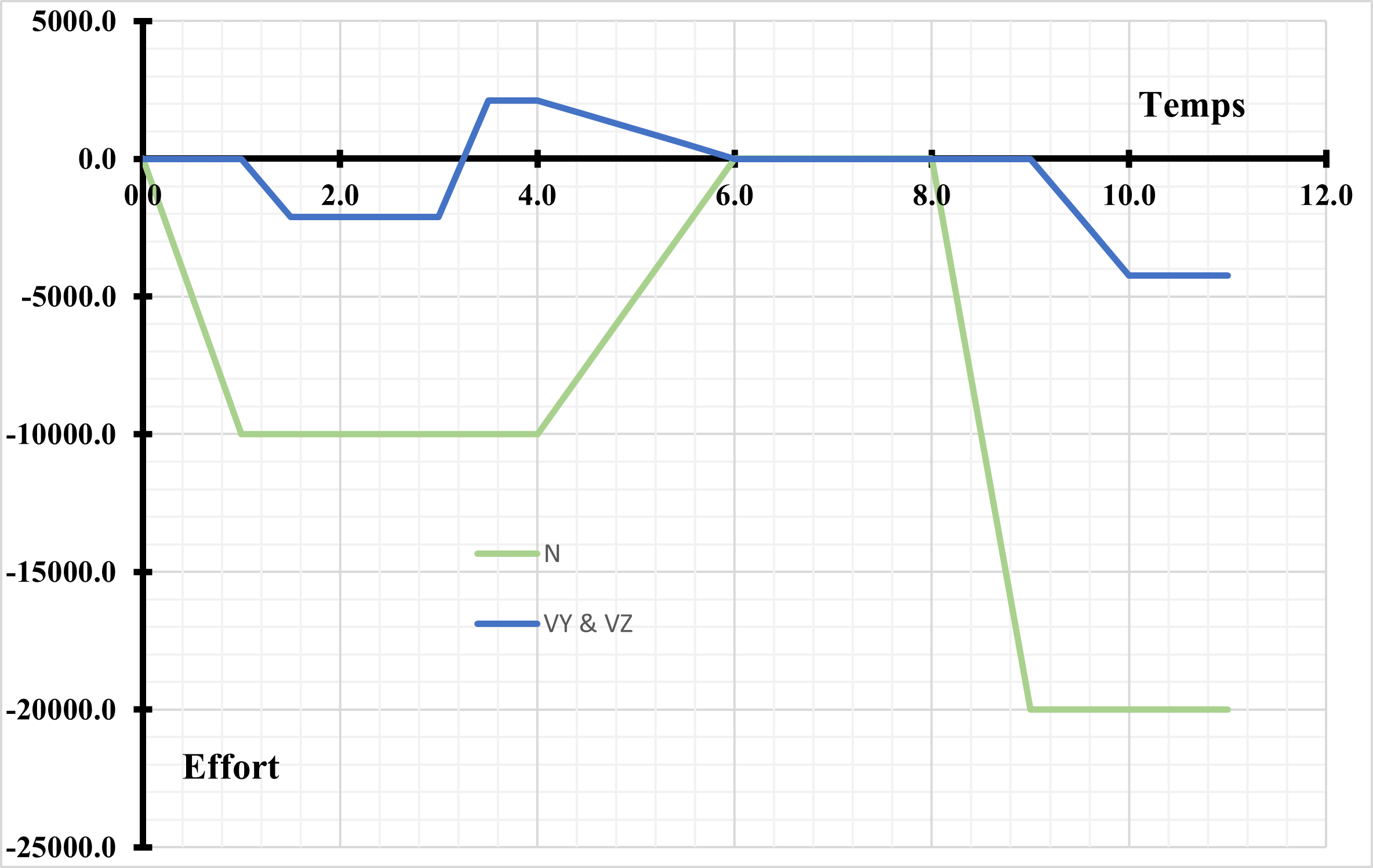
Figure 2.2.1.1-a :: Discreet efforts as a function of time . **
2.2.1.2. Charging path 2#
The forces in the tangential plane are verified for several angles:
\([\mathrm{0,30,45,60,90,120,135,150,180,210,225,240,270,300,315,330,360}]\)
The forces in the tangential plane are given by the following expressions:
\({V}_{Y}=\text{RIGI\_NOR}\phantom{\rule{2em}{0ex}}.{D}_{x}\mathrm{\mu }\mathrm{sin}(\mathit{Angle})\)
\({V}_{z}=\text{RIGI\_NOR}\phantom{\rule{2em}{0ex}}.{D}_{x}\mathrm{\mu }\mathrm{cos}(\mathit{Angle})\)
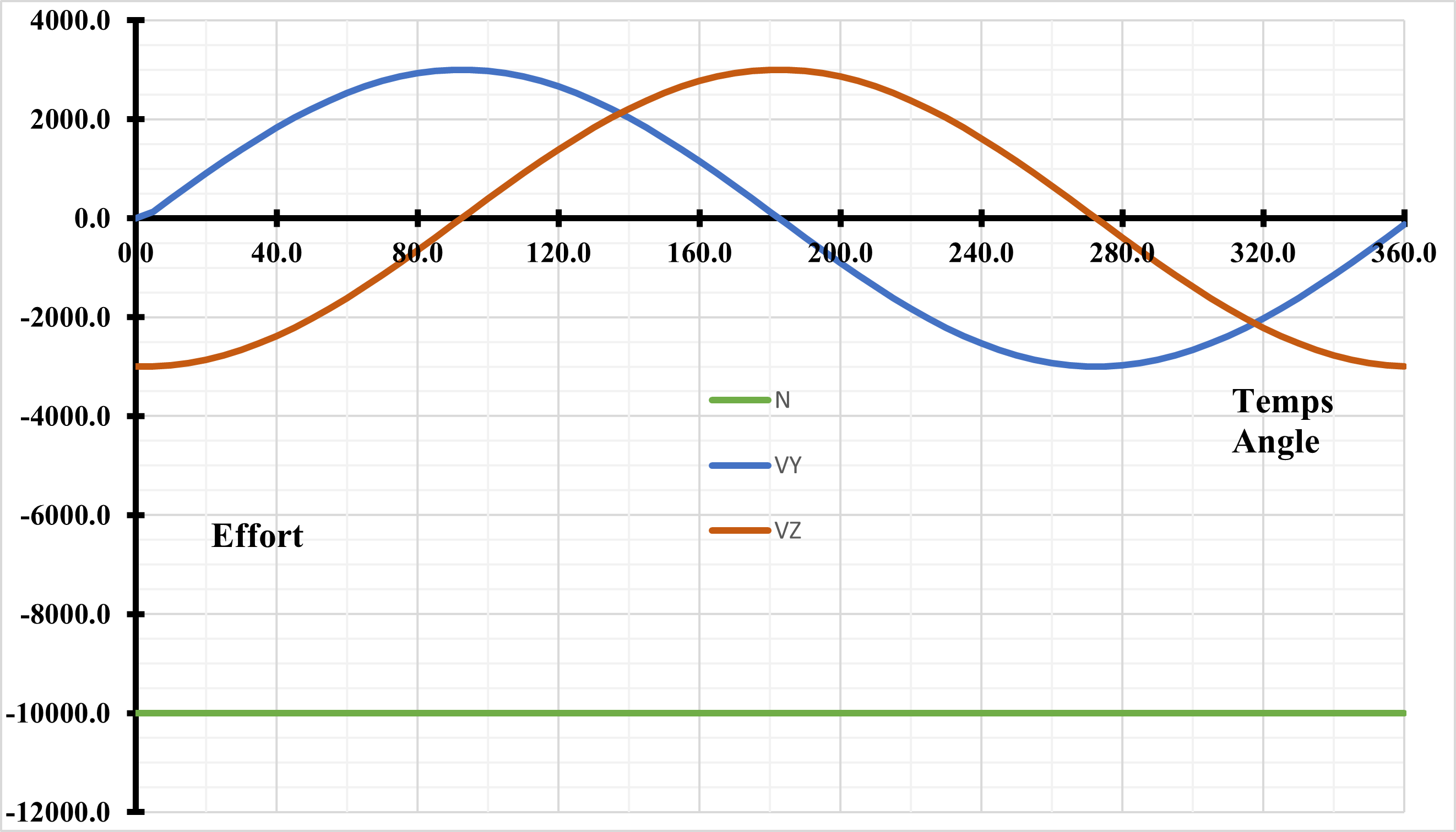
Figure 2.2.1.2-a :: Discreet efforts as a function of time . **
2.2.2. Uncertainty about solutions#
No uncertainty (analytical solutions).