1. Reference issues#
1.1. Geometry#
Discreet ones, like POI1 or SEG2 with a behavior like DIS_CONTACT.
1.2. Modeling A#
This case models a discrete elastic in parallel with a discrete shock.
1.2.1. Material properties#
Stiffness of the discrete elastic K_T_D_L, in coordinate system GLOBAL: (\({K}_{\mathit{el}}\), \({K}_{\mathit{el}}\) ,0) with \({K}_{\mathit{el}}=1\)
For the discreet DIS_CONTACT
RIGI_NOR \({K}_{n}\) |
1.0 |
RIGI_TAN \({K}_{t}\) |
0.5 |
COULOMB \(\mu\) |
0.5 |
DIST_1 |
0.5 |
DIST_2 |
0.0 |
Table 1.2.1-a: Material parameters of the shock discrete
1.2.2. Boundary conditions and loads#
One end is recessed.
The other end:
\(\mathit{DZ}=0\),
\(\mathit{FX}=-1\),
\(\mathit{FY}=2\).
Loads \(\mathit{FX}\) and \(\mathit{FY}\) are affected by the following time functions:
Time |
Affecting Function \(\mathit{FX}\) |
Affecting Function \(\mathit{FY}\) |
0.0 |
0.0 |
0.0 |
1.0 |
1.0 |
0.0 |
1.5 |
1.0 |
1.0 |
2.0 |
1.0 |
0.0 |
Table 1.2.2-a: Load multiplier functions
1.3. B modeling#
This case models a discrete like SEG2.

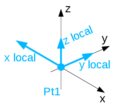
|
\(\mathit{Pt}1=(\mathrm{0.0,}\mathrm{0.0,}0.0)\) \(\mathit{Pt}2=(\mathrm{1.0,}\mathrm{0.0,}0.0)\) \(L1\mathrm{:}(\mathit{PT}\mathrm{1,}\mathit{PT}2)\) |
1.3.1. Material properties#
The behavior of the discrete is DIS_CONTACT, the material is DIS_CONTACT.
For loading path 1:
MAT1 = DEFI_MATERIAU (
DIS_CONTACT = _F (RIGI_NOR = 10000.0, 10000.0, RIGI_TAN =**20000.0,** COULOMB =** 0.3,
AMOR_TAN = 10.0, DIST_1 = 0.5, DIST_2 = 0.5 ),
)
The length of the discrete is \(1m\), with DIST_1 and DIST_2 taken into account, it is initially in contact without creating any effort.
For loading path 2:
MAT2 = DEFI_MATERIAU (
DIS_CONTACT = _F (RIGI_NOR = 10000.0, 10000.0, RIGI_TAN =**20000000.0,** COULOMB =** 0.3,
AMOR_TAN = 10.0, DIST_1 = 0.5, DIST_2 = 0.5 ),
)
The length of the discrete is \(1m\), with DIST_1 and DIST_2 taken into account, it is initially in contact without creating any effort.
For loading path 3:
MAT1 = DEFI_MATERIAU (
DIS_CONTACT = _F (RIGI_NOR = 10000.0, 10000.0, RIGI_TAN =**20000.0,** COULOMB =** 0.3,
AMOR_TAN = 10.0, DIST_1 = 0.5, DIST_2 = 0.75 ),
)
The length of the discrete is \(1m\), with DIST_1 and DIST_2 taken into account, it is initially in contact with the creation of an effort corresponding to a depression of \(0.25m\)
1.3.2. Boundary conditions and loads#
Node \(\mathit{Pt}2\) is stuck.
At node \(\mathit{Pt}1\), displacements are imposed according to the following time \(X,Y,Z\).
1.3.2.1. Loading path no. 1#
Table 1.3.2.1-a: Loading functions 1.
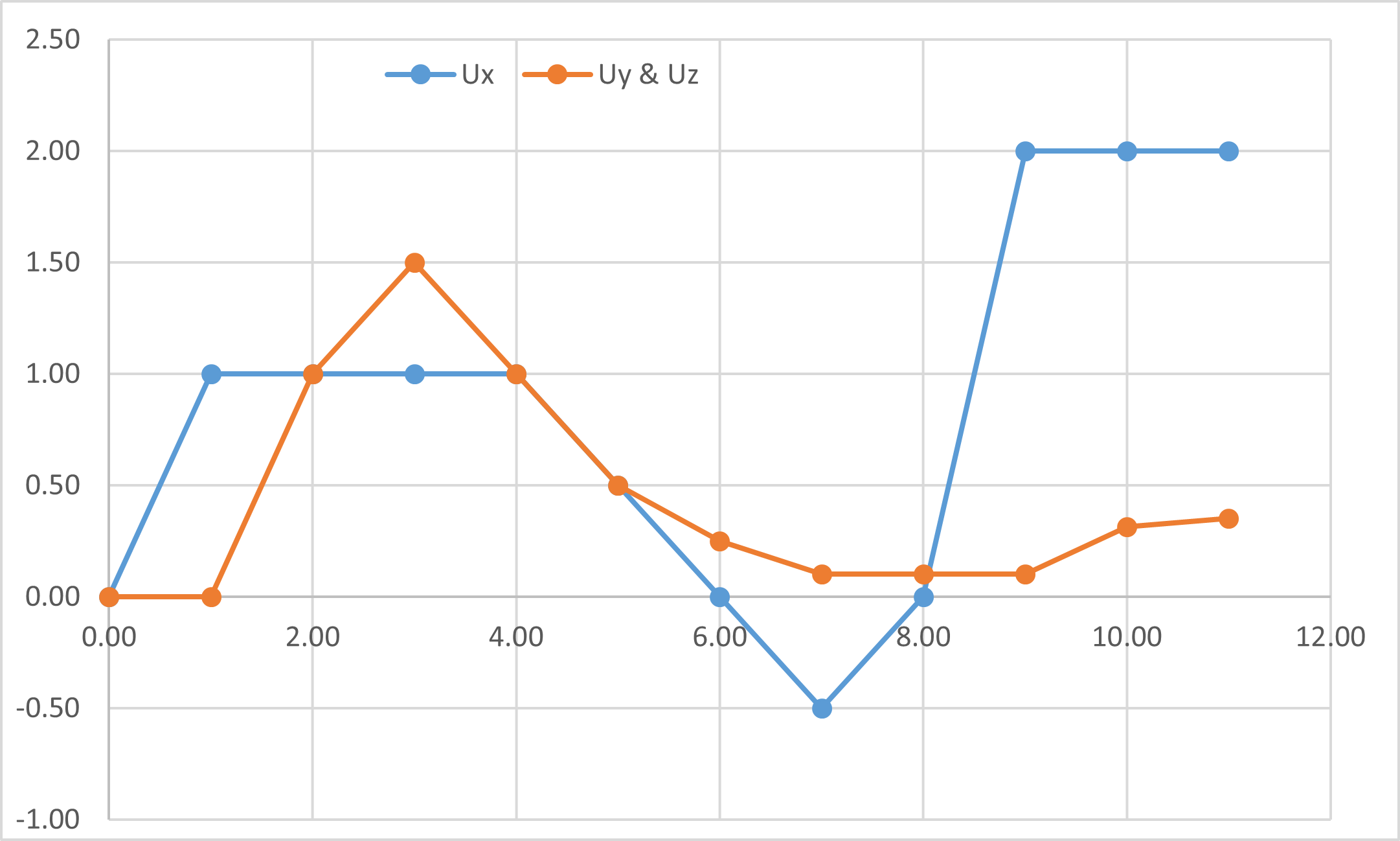
Figure 1.3.2.1-a : Charging path no**.**
With:
\(\mathit{Ux}\) represents the displacement in the discrete axis. A negative displacement corresponds to the « detachment » of the discrete.
\(\mathit{Uy},\mathit{Uz}\) represents the displacement in the tangential plane to the discrete.
1.3.2.2. Loading path no. 2#
This path is circular and makes it possible to verify that the frictional force is in the direction of the speed of movement.
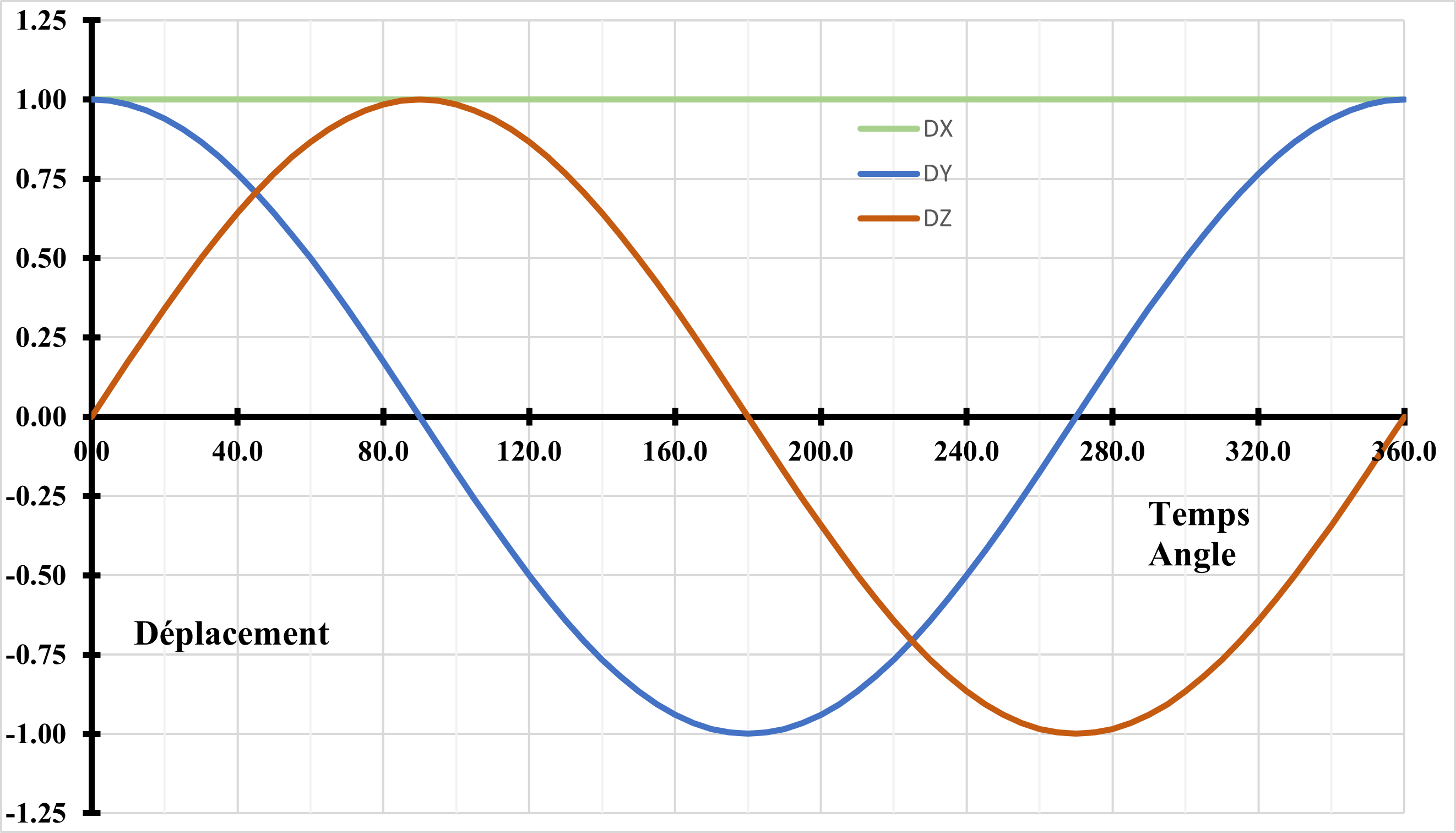
Figure 1.3.2.2-a : Loading path no.2 .
With:
\(\mathit{Dx}\) represents the displacement in the discrete axis. The discreet is always in contact.
\(\mathit{Dy},\mathit{Dz}\) represents the displacement in the tangential plane to the discrete.
1.3.2.3. Loading path no. 3#
This path corresponds to path No. 1 in the tangential plane. As this discrete is initially pressed from \(0.25m\), the movement along the \(X\) axis is offset by \(-0.25m\) to obtain the same results.
1.4. C modeling#
This case models a discrete like POI1.
The material properties and the loading paths are identical to those of the B model.