1. Reference problem#
1.1. Geometry#
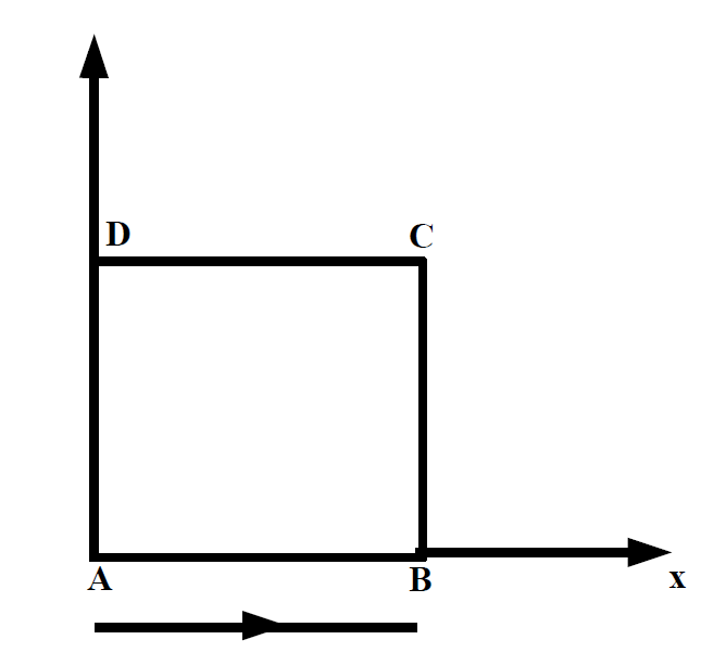
Figure 1.1-a
The geometry refers to a single finite isoparametric element of square shape, the length of each edge is equal to 1.
1.2. Material properties#
The mass consists of an elasto-plastic material modelled by a Drucker Prager law of behavior, associated or not.
The material elasticity parameters are as follows:
Isotropic elasticity Young’s modulus: \(E={10}^{9}\mathrm{Pa}\)
Poisson’s ratio: \(\nu \mathrm{=}\mathrm{0,3}\)
Real constant density: \(\mathrm{\rho }=2764\mathit{kg}\mathrm{.}{m}^{-3}\)
Isotropic thermal expansion coefficient: \(\alpha =0\)
The characteristics of work hardening are then given by:
Pressure dependence coefficient: \(\alpha =\mathrm{0,328}\)
Elastic limit: \({\sigma }_{y}\mathrm{=}2.11\mathrm{\times }{10}^{6}\)
Ultimate constraint: \({\mathrm{\sigma }}_{\mathit{ULTM}}=1.0\times {10}^{6}\)
For modeling A:
Ultimate cumulative plastic deformation: \({P}_{\mathrm{ULT}}=2\)
For B modeling:
Ultimate cumulative plastic deformation: \({P}_{\mathit{ULT}}\mathrm{=}1.225\mathrm{\times }{10}^{\mathrm{-}2}\)
1.3. Boundary conditions and loads#
A unit displacement is imposed along the \(y\) axis on the \(\mathrm{CD}\) segment, zero along the \(y\) axis on the \(\mathrm{AB}\) segment and zero along the \(x\) axis on the \(\mathrm{AD}\) segment.
In this test case, concerning modeling A, we simulate a case of perfect plasticity with the two Drucker-Prager behavior laws in associated and non-associated conditions to verify the computational consistency of the results. To do this, simply take large values for \({P}_{\mathit{ULT}}\).