2. Benchmark solution

2.1. Calculation method

We do not have an exact analytical solution for this problem. The reference solutions are taken from the literature (cf. 1, p.262). They are numerical solutions obtained by finite element calculations.

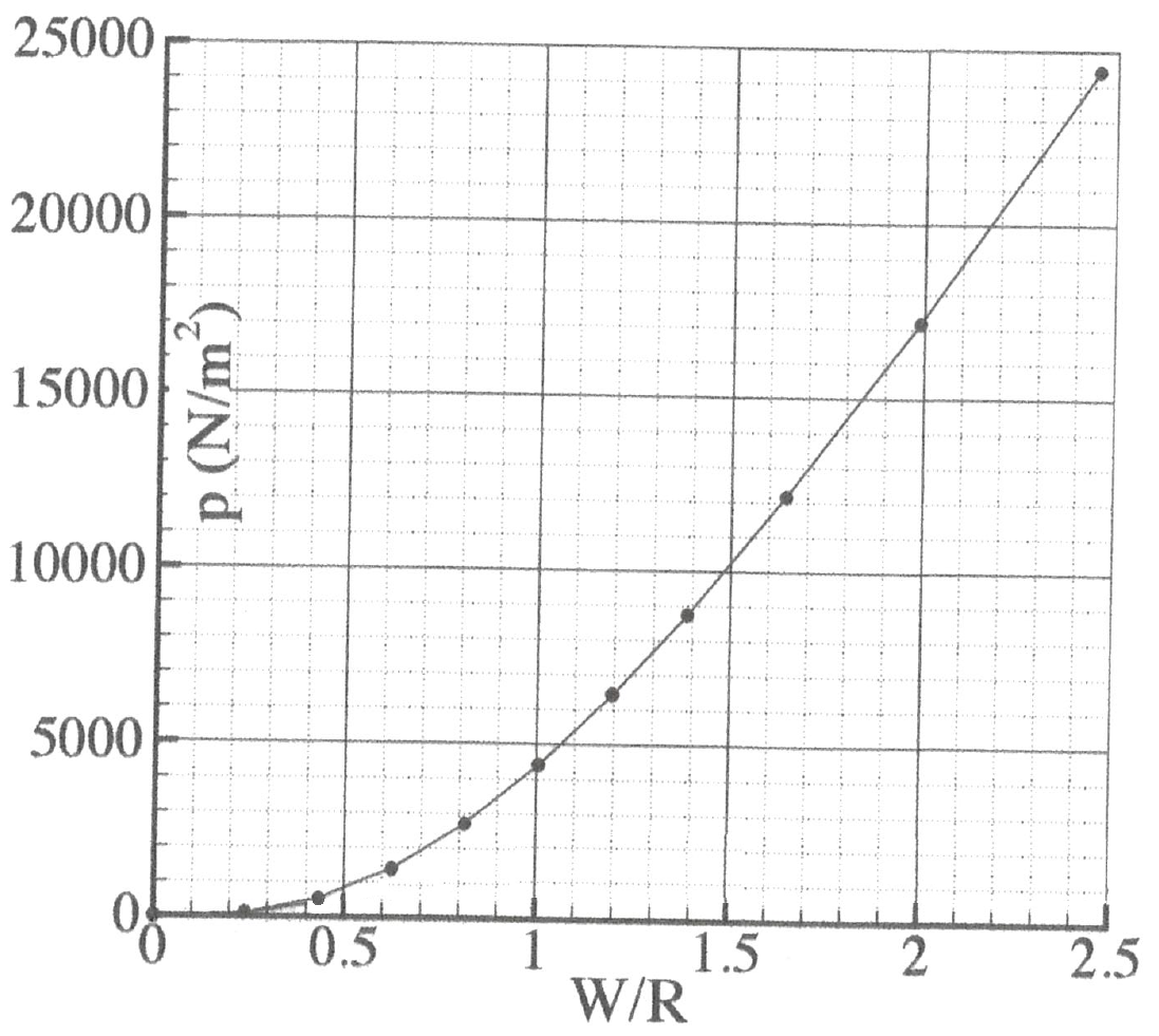
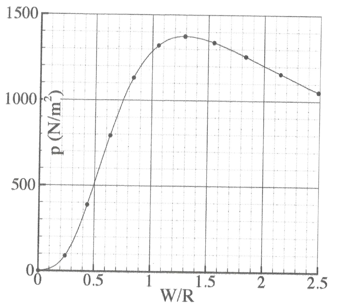
Figure 2.1-a: Reference curves for the laws of Saint Venant Kirchhoff (on the left) and Neo-Hookaean (on the right).

2.2. Reference quantities and results

For the law of Saint Venant Kirchhoff, we test the vertical displacement at point O at the final moment. The displacement is obtained on the left curve in FIG. 2.1-a:

Size	Identification	Law of Behavior	Reference Solution
Displacement	Instant 1.0 - Point \(O\) - \(\mathit{DZ}\)	Saint Venant Kirchhoff	2448 \(\mathit{mm}\)

For the Neo-Hookean law of behavior, the pressures are interpolated at each moment of calculation on the right curve in Figure 2.1-a:

Size	Identification	Law of Behavior	Reference Solution
Pressure	Instant 0.1 - \(\mathit{ETA}\text{\_}\mathit{PILO}\)	Neo-Hookean	109.55 \(N/{m}^{2}\)
Pressure	Instant 0.2 - \(\mathit{ETA}\text{\_}\mathit{PILO}\)	Neo-Hookean	531.73 \(N/{m}^{2}\)
Pressure	Instant 0.3 - \(\mathit{ETA}\text{\_}\mathit{PILO}\)	Neo-Hookean	995.8 \(N/{m}^{2}\)
Pressure	Instant 0.4 - \(\mathit{ETA}\text{\_}\mathit{PILO}\)	Neo-Hookean	1276.2 \(N/{m}^{2}\)
Pressure	Instant 0.5 - \(\mathit{ETA}\text{\_}\mathit{PILO}\)	Neo-Hookean	1366.9 \(N/{m}^{2}\)
Pressure	Instant 0.6 - \(\mathit{ETA}\text{\_}\mathit{PILO}\)	Neo-Hookean	1344.7 \(N/{m}^{2}\)
Pressure	Instant 0.7 - \(\mathit{ETA}\text{\_}\mathit{PILO}\)	Neo-Hookean	1280.6 \(N/{m}^{2}\)
Pressure	Instant 0.8 - \(\mathit{ETA}\text{\_}\mathit{PILO}\)	Neo-Hookean	1203.0 \(N/{m}^{2}\)
Pressure	Instant 0.9 - \(\mathit{ETA}\text{\_}\mathit{PILO}\)	Neo-Hookean	1124.4 \(N/{m}^{2}\)
Pressure	Instant 1.0 - \(\mathit{ETA}\text{\_}\mathit{PILO}\)	Neo-Hookean	1049.0 \(N/{m}^{2}\)

2.3. Uncertainties about the solution

The reference solution is digital. The reference mesh is composed of 196 elements of type QUAD8.

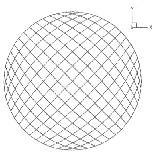
Figure 2.3-a: Reference solution mesh.

Some differences in the solutions obtained can be explained by differences in meshes. In addition, the values were recorded using the G3Data Graph Analyzer software on a scan of a graph contained in the reference book. Uncertainty is therefore directly linked to the quality and precision of printing the book, as well as to the precision of the scores made.

2.4. Bibliographical references

1. 1. LE VAN: Shells and membranes, the foundation of the nonlinear approach. Technosup (2014).