1. Reference problem#
1.1. Geometry#
We consider a reinforced concrete column of length \(\mathrm{0,7}m\), along the axis \(\mathrm{Ox}\), with a square cross section with a height and width equal to \(\mathrm{0,15}m\).
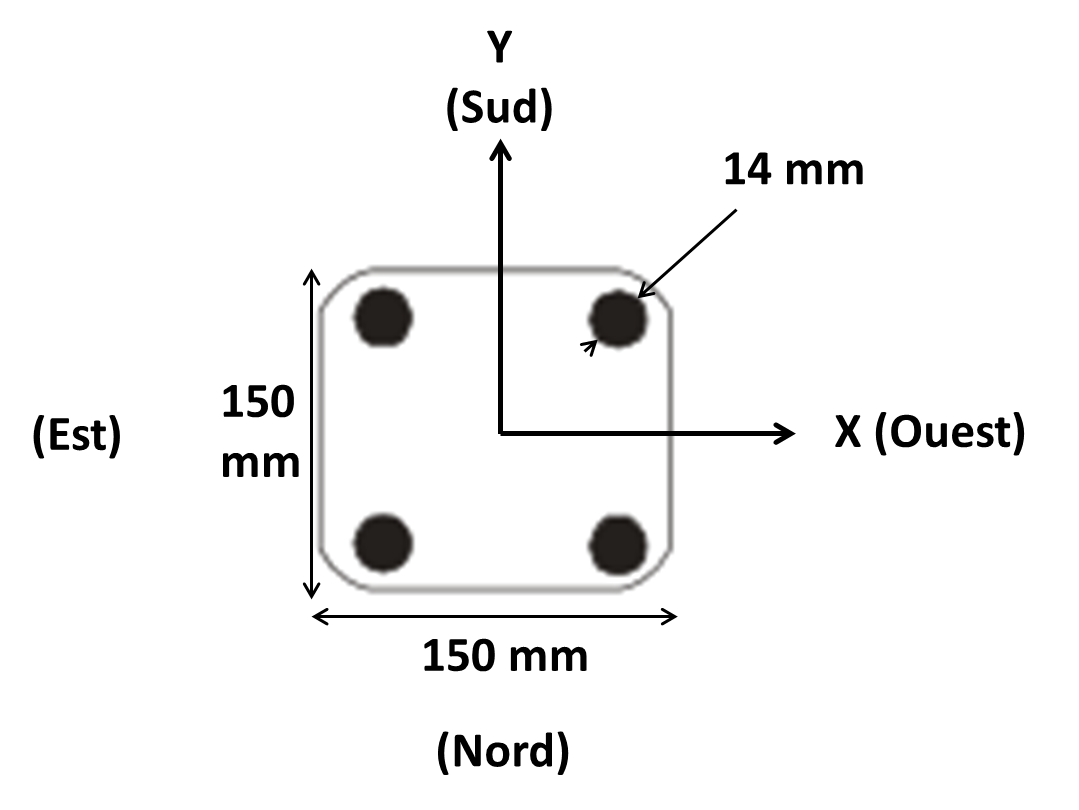
Figure 1: reinforced concrete column section.
The longitudinal frames are four \(\mathit{HA14}\).
The transverse reinforcements are not taken into account in the models below.
For modeling A, two reinforcing bars \(X\) and \(Y\) from \(\mathrm{2,053}\text{}{10}^{-3}{m}^{2}/m\) are used.
For modeling B, a single steel fiber with section \(\mathrm{6,15}{\mathit{mm}}^{2}\) is used.
1.2. Material properties#
The GLRC_DM law of behavior has the following parameters for concrete:
Young’s modulus: \(E\mathrm{=}28500\mathit{MPa}\)
Poisson’s ratio: \(\nu \mathrm{=}0.2\)
Maximum compression stress: \({\sigma }_{c}=25\mathrm{MPa}\)
Peak deformation under compression: \({ϵ}_{c}=\mathrm{2,25}\mathrm{.}\text{}{10}^{-3}\)
Maximum tensile stress: \({\sigma }_{t}=\mathrm{2,94}\mathit{MPa}\)
The parameters for steel are:
Young’s modulus: \(E\mathrm{=}195000\mathit{MPa}\)
Poisson’s ratio: \(\nu \mathrm{=}0.3\)
Elastic limit: \({\sigma }_{y}=610\mathrm{MPa}\)
Tangent module (plastic slope): \({E}_{t}\mathrm{=}\mathrm{19,5}\mathit{MPa}\)
The operator DEFI_GLRC is used to obtain the parameters of the GLRC_DM law. Concrete stress has been reduced to \({\sigma }_{t}=\mathrm{1,6}\mathit{MPa}\). In addition, the parameters \({\gamma }_{c}=\mathrm{0,35}\) and \({\alpha }_{c}=60\) are also set for the non-linear behavior in compression.
With these material data, the equivalent elastic modulus in membrane, cf. [R7.01.32], is equal to: \({E}_{\mathrm{eq}}^{m}=34021.0\mathrm{MPa}\), i.e. membrane stiffness in the direction \(\mathrm{Ox}\): \({E}_{\mathrm{eq}}^{m}\ast S=765.393\mathrm{MN}\).
The DEFI_MATER_GC operator was used to determine the parameters of laws MAZARS_UNIL and VMIS_CINE_GC.
1.3. Boundary conditions and loads#
One end of the beam, edge \(A\), is blocked and a distributed force of the resultant \(\mathit{FX}\mathrm{=}1\mathit{kN}\) is imposed on the other end, edge \(B\), in the direction \(X\).
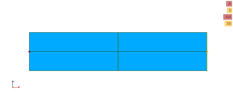
Figure 2: reinforced concrete column section.
Charging cycles are defined by:
\(t\) |
Multiplying factor on the \(\mathit{FX}\) force |
\(\mathrm{0,0}\) |
|
\(\mathrm{1,0}\) |
|
\(\mathrm{3,0}\) |
|
\(\mathrm{5,0}\) |
|
\(\mathrm{7,0}\) |
|
\(\mathrm{9,0}\) |
|
\(\mathrm{11,0}\) |
|
\(\mathrm{13,0}\) |
|
\(\mathrm{15,0}\) |
|
\(\mathrm{17,0}\) |
|
\(\mathrm{19,0}\) |
|
1.4. Initial conditions#
Nil.