2. Benchmark solution#
The modeling verifies the behavior of the linear hardening law.
2.1. Calculation method#
The equations we are interested in for analytical calculation are (\({I}_{1}=\text{tr}(\sigma )\): stress tensor trace, \({\varepsilon }_{v}^{p}\): volume plastic deformation):
plastic constitutive law on the volume part:
: label: EQ-None
{I} _ {1} =mathrm {3K} ({varepsilon} _ {v} - {varepsilon} _ {v} ^ {p})
criterion area, setting the Von Mises constraint to zero (\({\sigma }_{\mathrm{eq}}=0\)):
: label: EQ-None
F (sigma, p) =alpha {I} _ {1} -R (p)
relationship between volume plastic deformation and cumulative plastic deformation (internal plastic law variable):
: label: EQ-None
dot {{varepsilon} _ {v}} ^ {p}} =3alphadot {p}
expression of work hardening
linear:
: label: EQ-None
begin {array} {} R (p) = {sigma} _ {Y}} _ {Y} +hpmathrm {si} ple {p} _ {mathrm {ult}}}\ R (p) = {sigma} = {sigma}} = {mathrm {ult}}} = {sigma} _ {Y}} ^ {mathrm {ult}} ^ {mathrm {ult}} ^ {mathrm {ult}} ^ {mathrm {ult}} ^ {mathrm {ult}} ^ {mathrm {ult}} ^ {mathrm {ult}} ^ {mathrm {ult}} ^ {mathrm {ult}} ^ {mathrm {ult}}}mathrm {si} p > {p} _ {mathrm {ult}}end {array}
parabolic:
: label: EQ-None
begin {array} {} R (p) = {sigma} _ {Y}} {(1- (1-sqrt {sigma} _ {Y} ^ {mathrm {ult}}}}} {{sigma}}}} {{sigma}}}} {{sigma} _ {sigma}}}} {{sigma}}}}} {{sigma}}}} {{sigma}}}} {{sigma}}}} {{sigma}}}} {{sigma}}}} {{sigma}}}} {{sigma} _ {Y}}}) {{sigma} _ {Y}}}) {{sigma}}}} {{sigma}}}} {{sigma}}}} {{sigma} thrm {si} ple {p} _ {mathrm {ult}} {mathrm {ult}}}\ R (p) = {sigma} _ {Y} ^ {mathrm {ult}}}mathrm {ult}}\ mathrm {ult}}end {ult}}end {array}}mathrm {ult}}
We observe that, as in the linear case, \(R(p)={\sigma }_{Y}\) if \(p=0\) and we have perfect plasticity if \(p>{p}_{\mathrm{ult}}\).
2.1.1. Deformation at the initial elastic limit#
This deformation is obtained for \({\varepsilon }_{v}^{p}=p=0\).
If we ask \(F(\sigma ,p)=0\) (plastic evolution) we have:
\({I}_{1}^{\mathrm{el}}=\frac{R(p)}{\alpha }=\frac{{\sigma }_{Y}}{\alpha }\)
\({\varepsilon }_{v}^{\mathrm{el}}=\frac{{I}_{1}^{\mathrm{el}}}{3K}\)
2.1.2. Ultimate deformation#
The ultimate deformation \({\varepsilon }_{v}^{\mathrm{ult}}\) is called the one obtained for \(p={p}_{\mathrm{ult}}\).
The corresponding stress trace \({I}_{1}^{\mathrm{ult}}\) and the plastic deformation \({\varepsilon }_{v}^{\mathrm{pult}}\) can easily be found:
\({I}_{1}^{\mathrm{ult}}=\frac{R(p)}{\alpha }=\frac{{\sigma }_{Y}^{\mathrm{ult}}}{\alpha }\)
\({\varepsilon }_{v}^{\mathrm{pult}}=3\alpha {p}_{\mathrm{ult}}\)
\({\varepsilon }_{v}^{\mathrm{ult}}=\frac{{I}_{1}^{\mathrm{ult}}}{3K}+{\varepsilon }_{v}^{\mathrm{pult}}\)
2.1.3. Deformation between the elastic limit and the ultimate deformation#
First, the cumulative plastic deformation is calculated.
Combining equations (), (), () and () with :math:`F(sigma ,p)=0` for**linear work hardening* we have:
: label: EQ-None
p=frac {3KA {varepsilon} _ {mathrm {v1}} - {sigma} _ {Y}} {9K {alpha} ^ {2} +h}
By combining equations (), (), () and () with :math:`F(sigma ,p)=0` for**parabolic work hardening* we arrive at the equation of degree 2:
: label: EQ-None
{A} _ {1} {stackrel {} {p}}} ^ {2}} + {B} _ {1}stackrel {} {p} {p} + {C} _ {1} =0 begin {array} {} {A} _ {1} = {sigma} _ {1} _ {Y} {(1-gamma)} ^ {2}\ {B} _ {1} =9K {alpha} ^ {2} {2} {p} = {p} _ {p} _ {p} _ {p} _ {p} _ {p} _ {p} _ {p} _ {p} _ {p} _ {p} _ {p} _ {p} _ {p} _ {p} _ {p} _ {p} _ {p} _ {p} _ {p} _ {p} _ {p} _ {p} _ {p} _ {p} _ {p} _ {p} _ {p} _ {p} _ {p} _ {p} _ {sigma} _ {Y} -3Kalpha {varepsilon} _ {vtext {1}}\gamma =sqrt {frac {{sigma} _ {Y} ^ {mathrm {ult}}} {mathrm {ult}}}}} {{sigma}}} {{sigma} _ {Y}}}}\stackrel {} {p} {p}} =frac {p}} =frac {p} {p} _ {mathrm {ult}}}}end {array}
We then use the equations () () to find the plastic deformation \({\varepsilon }_{v}^{p}\) and the stress trace \({I}_{1}\).
If the material is unloaded elastically until zero stress is reached, a residual deformation equal to the plastic deformation is obtained; on the other hand, it is necessary to load the material under compression to obtain zero total deformation. This second branch is also elastic, because the Drücker-Prager material cannot plasticize in a state of hydrostatic compression. In the latter case, the negative stress trace is:
: label: EQ-None
{I} _ {1} ^ {c} =-3K {varepsilon} _ {v} ^ {p}
2.1.4. Deformation greater than ultimate deformation#
All the quantities of interest are easily found, because the constraint trace is known a priory and equal to \({I}_{1}^{\mathrm{ult}}\).
\({\varepsilon }_{v}^{p}={\varepsilon }_{v}-\frac{{I}_{1}^{\mathrm{ult}}}{3K}\)
\(p=\frac{{\varepsilon }_{v}^{p}}{3\alpha }\)
2.2. Reference quantities and results#
The compressibility module \(K\) is:
\(K=\frac{E}{3(1-2\nu )}=2000\mathrm{MPa}\)
2.2.1. Deformation at the elastic limit#
For both models we can easily find:
\({I}_{1}^{\mathrm{el}}=30\mathrm{MPa}\)
\({\varepsilon }_{v}^{\mathrm{el}}=\mathrm{0,005}\)
2.2.2. Ultimate deformation#
For both models we find:
\({I}_{1}^{\mathrm{ult}}=50\mathrm{MPa}\)
\({\varepsilon }_{v}^{\mathrm{pult}}=\mathrm{0,024}\)
\({\varepsilon }_{v}^{\mathrm{ult}}\approx \mathrm{0,03233}\)
2.2.3. Deformation equal to 0.018 and zero deformation discharge#
This deformation value \({\varepsilon }_{v\text{1}}=\mathrm{0,018}\) is greater than the elastic limit \({\varepsilon }_{v}^{\mathrm{el}}\) and less than \({\varepsilon }_{v}^{\mathrm{ult}}\). We first calculate the cumulative plastic deformation with the equations () and (), then the plastic deformation and the stress trace:
linear work hardening:
\({p}_{1}=\frac{3KA{\varepsilon }_{\mathrm{v1}}-{\sigma }_{Y}}{9K{\alpha }^{2}+h}\approx \mathrm{0,019}\)
\({\varepsilon }_{v\text{1}}^{p}=3\alpha {p}_{1}=\mathrm{0,0114}\)
\({I}_{1}^{1}=3K({\varepsilon }_{v\text{1}}-{\varepsilon }_{v\text{1}}^{p})\approx \mathrm{39,51}\mathrm{MPa}\)
parabolic work hardening:
\({p}_{1}\approx 0.0192\)
\({\varepsilon }_{v\text{1}}^{p}=3\alpha {p}_{1}\approx 0.0115\)
\({I}_{1}^{1}=3K({\varepsilon }_{v\text{1}}-{\varepsilon }_{v\text{1}}^{p})\approx 38.956\mathrm{MPa}\)
The zero deformation stress trace is:
linear work hardening:
\({I}_{1}^{\mathrm{1c}}=-3K{\varepsilon }_{v\text{1}}^{p}\approx -\mathrm{68,49}\mathrm{MPa}\)
parabolic work hardening:
\({I}_{1}^{\mathrm{1c}}=-3K{\varepsilon }_{v\text{1}}^{p}\approx -\mathrm{69,044}\mathrm{MPa}\)
Indeed, the difference between the parabolic and linear case is very small.
2.2.4. Loading until deformation equal to 0.045 and 0.06#
The material is recharged up to deformation values \({\varepsilon }_{v\text{2}}=\mathrm{0,045}\) and \({\varepsilon }_{v\text{3}}=\mathrm{0,06}\), which are greater than \({\varepsilon }_{v}^{\mathrm{ult}}\).
The results are the same for both models.
For \({\varepsilon }_{v\text{2}}=\mathrm{0,045}\):
\({\varepsilon }_{v\text{2}}^{p}={\varepsilon }_{v\text{2}}-\frac{{I}_{1}^{\mathrm{ult}}}{3K}\approx \mathrm{0,03667}\)
\({p}_{2}=\frac{{\varepsilon }_{v\text{2}}^{p}}{3\alpha }\approx \mathrm{0,0611}\)
Following the elastic discharge (up to zero stress), we find \({\varepsilon }_{v}={\varepsilon }_{v\text{2}}^{p}\), \(p={p}_{2}\).
For \({\varepsilon }_{v\text{3}}=\mathrm{0,06}\):
\({\varepsilon }_{v\text{3}}^{p}={\varepsilon }_{v\text{3}}-\frac{{I}_{1}^{\mathrm{ult}}}{3K}\approx \mathrm{0,051667}\)
\({p}_{3}=\frac{{\varepsilon }_{v\text{3}}^{p}}{3\alpha }\approx \mathrm{0,0861}\)
2.2.5. Stress-strain curves#
In Figures () and () the curve (\({\varepsilon }_{v},{I}_{1}\)) for linear and parabolic work hardening is represented. In red are the points tested by the test case.
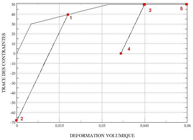
Figure 2.2.5-a : stress-strain curves for linear work hardening.
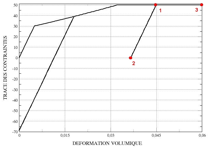
Figure 2.2.5-b : stress-strain curves for parabolic work hardening.
2.3. Uncertainty about the solution#
The solution is analytical.
2.4. Bibliographical references#
Document [R3.01.16], Integration of the elasto-plastic mechanical behavior of Drücker-Prager DRUCK_PRAGER and post-treatments. Code_Aster reference manual.