2. Benchmark solution#
2.1. Calculation method#
Analytical solution for damage variable \(D\):
\(D(t)\mathrm{=}1\mathrm{-}{(1\mathrm{-}(1+k){(\frac{{\sigma }_{0}}{A})}^{R}t)}^{\frac{1}{1+k}}\)
Analytical solution for the viscoplastic isotropic work hardening variable, \(r\), in the case of a zero \({\sigma }_{Y}\) threshold:
\(r(t)\mathrm{=}{\left[\frac{(M+N)}{M(1+k\mathrm{-}N)}{(\frac{{\sigma }_{0}}{A})}^{\mathrm{-}R}{(\frac{{\sigma }_{0}}{K})}^{N}(1\mathrm{-}{(1\mathrm{-}(1+k){(\frac{{\sigma }_{0}}{A})}^{R}t)}^{\frac{1+k\mathrm{-}N}{1+k}})\right]}^{\frac{M}{M+N}}\)
In the previous expressions, \(D\) is the damage variable corresponding to the internal variable \(\mathit{V9}\) and \(r\) is the multiplicative viscoplastic work hardening variable corresponding to the internal variable \(\mathit{V8}\).
We also have the following correspondence, in relation to the parameters of the VENDOCHAB keyword:
\(N\mathrm{=}{N}_{\mathit{VP}}\)
\(M\mathrm{=}{M}_{\mathit{VP}}\)
\(K\mathrm{=}{K}_{\mathit{VP}}\)
\(A\mathrm{=}{A}_{D}\)
\(R\mathrm{=}{R}_{D}\)
\(k\mathrm{=}{K}_{D}\)
2.2. Reference quantities and results#
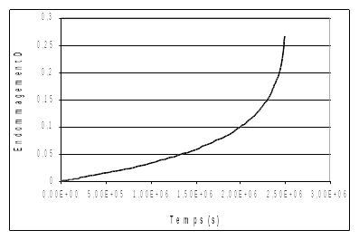
Evolution of the damage variable, \(D\), as a function of time. This value is tested at various times:
Instant |
Reference |
520000 |
1.52596E-02 |
1000000 |
3.30676E-02 |
2000000 |
9.9465369E-02 |
2250000 |
1.37520763E-01 |
2500000 |
2.66018229E-01 |
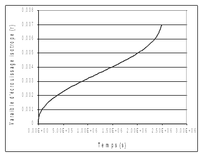
Evolution of the viscoplastic isotropic work hardening variable, \(r\), as a function of time. This value is tested at various times:
Instant |
Reference |
520000 |
2.300147E-03 |
1000000 |
3.179469E-03 |
2000000 |
4.95103E-03 |
2250000 |
5.592847E-03 |
2500000 |
6.99749E-03 |
The difference observed on \(D\) for \(t=2.5{10}^{6}s\) is due to the very high non-linearity of the evolution of the damage variable.
2.3. Uncertainties about the solution#
Code accuracy