1. Reference problem#
1.1. Geometry#
Structure \(\mathrm{2D}\) is a rectangular specimen (\(\mathit{LX}=10\), \(\mathit{LY}=20\)), with a straight and horizontal central crack []. The half-length of the crack is constant (\(a=1\)).
The 3D structure corresponds to an extrusion in the Z direction of the 2D specimen. The test piece becomes parallelepipedic in dimensions: \(\mathit{LX}=10\), \(\mathit{LY}=20\), \(\mathit{LZ}=1\). The crack of length \(a=1\) in the plane (X, Y) is also extruded along Z.
The nodes marked \(\mathit{NOEUD1}\), \(\mathit{NOEUD2}\) on the serve to impose boundary conditions, which are explained in paragraph [§ 1.3].
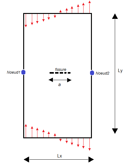
Figure 1.1-1:2D cracked plate geometry
1.2. Material properties#
Young’s module: \(E={10}^{6}\mathit{Pa}\)
Poisson’s ratio: \(\nu =0\)
Density: \(\rho =7800\mathrm{kg}/{m}^{3}\)
1.3. Boundary conditions and loads#
2D problem (A, B, C, D models) :
Loading consists in applying a linear force density, distributed over the lower and upper edges of the specimen [].
On the upper edge we apply a force density: \({F}_{1}(X,Y)=X\)
On the lower edge we apply a force density: \({F}_{2}(X,Y)=-X\)
This load exerts a compression on one half of the test piece (half on the left), a pull on the other half of the test piece (half on the right). This results in a flexure of the test piece [].
Thanks to this load, we impose:
the closure of the crack, in the vicinity of the bottom of crack \(\mathit{P1}=(-a\mathrm{,0})\), contained in half of the specimen under compression;
the opening of the crack, in the vicinity of the bottom of crack \(\mathit{P2}=(a\mathrm{,0})\), contained in half of the test specimen under tension (see [])
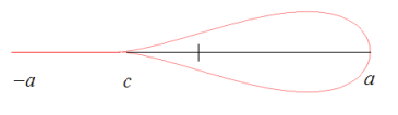
Figure 1.3-1: Partially closed crack
In order to block rigid modes, we block the movements of nodes \(\mathit{NOEUD1}\), \(\mathit{NOEUD2}\) as follows:
\({\mathit{DX}}^{1}={\mathit{DY}}^{1}=0\)
\({\mathit{DY}}^{2}=0\).
This blocking is applied taking into account the field of movement []. In fact, the displacement is strictly zero at the nodes in question, because they belong to the plane of symmetry of the test piece, around which the test piece bends.
3D problem (E, F, G, models) :
The 3D problem includes all the boundary conditions of the 2D problem by adding only the Z direction:
the efforts on the upper side \({F}_{1}(X,Y,Z)=X\),
the efforts on the underside \({F}_{2}(X,Y,Z)=-X\),
the blocking of rigid modes \({\mathit{DX}}^{1}={\mathit{DY}}^{1}={\mathit{DZ}}^{1}=0\), \({\mathit{DX}}^{2}={\mathit{DY}}^{2}=0\) and a 3rd point in the plane of symmetry for the last rigid mode \({\mathit{DZ}}^{3}=0\).
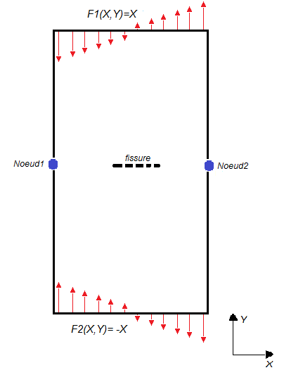
Figure 1.3-2: Boundary conditions of the 2D problem