4. B modeling#
4.1. Characteristics of modeling#
In this modeling, the extended finite element method (\(\text{X-FEM}\)) is used. We define an enrichment radius \({R}_{\mathit{ENRI}}=0.5\). Finite elements are linear.
4.2. Characteristics of the mesh#
Same as modeling A.
4.3. Tested sizes and results#
On the background of the crack in opening \(P2=(a\mathrm{,0})\), the stress intensity factor \({K}_{I}\) given by the command CALC_G is tested, compared to the analytical value explained in paragraph [5].
For method \(G-\mathit{thêta}\) (command CALC_G), the following crowns of the theta field are chosen:
Crown 1 |
Crown 2 |
Crown 3 |
Crown 3 |
Crown 4 |
Crown 5 |
Crown 6 |
|
Rinf |
0.1 |
0.2 |
0.2 |
0.3 |
0.3 |
0.1 |
0.2 |
Rsup |
0.2 |
0.3 |
0.3 |
0.3 |
0.4 |
0.4 |
0.4 |
Identification |
Reference type |
Reference value |
Precision |
|
CALC_G /K1 |
“ANALYTIQUE” |
0.9648 |
|
|
CALC_G /K2 |
“ANALYTIQUE” |
0.00 |
0.00 |
0.001 |
CALC_G /G |
“ANALYTIQUE” |
9.3084E-7 |
|
4.4. Additional results#
By activating the contact algorithm, we obtain the solution moving in the vicinity of the crack given to [] (to be compared with post-treatment).
On the other hand, we find an analytical conclusion, namely the abscissa of the point at which the crack begins to open:
\(c=-\frac{a}{3}\approx -0.33\)
Indeed, in post-treatment, we analyzed the contact pressures to determine the abscissa of the last point of contact. Graphically, it is estimated that the pressure falls sharply around the abscissa point \({x}_{c}\approx -0.325\), which validates the estimation hypothesis of \({K}_{I}\).
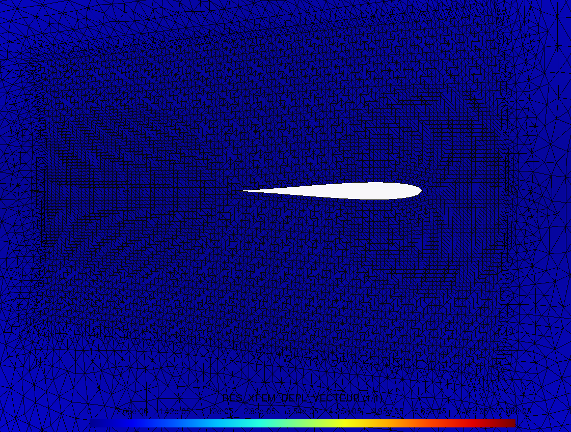
Figure 4.4-1: contact crack closure facies
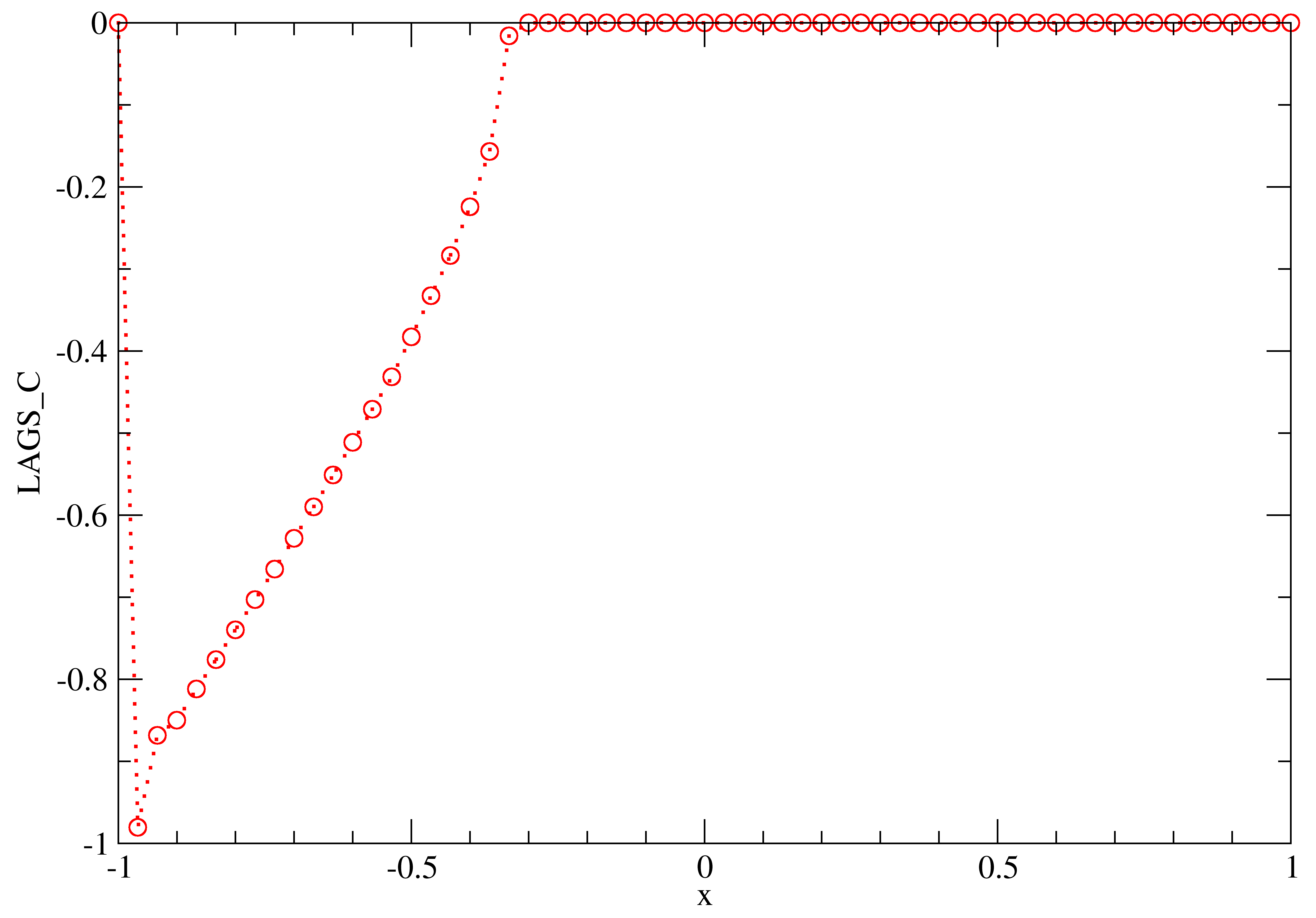
Figure 4.4-2: contact pressure along the crack