1. Reference problem#
1.1. Geometry#
The geometry of the test case studied consists of a rectangular plate with a hole in its center subjected to traction.
For obvious reasons of symmetry, only a quarter of the plate is studied.
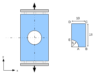
Figure 1.1-a : Problem studied
1.2. Material properties#
Since the objective is to test the different laws of behavior, the different models use different laws of behavior.
In the case of models \(A\), \(B\) and \(E\), the material that constitutes the plate is modelled by an elastoplastic behavior law. The plasticity criterion is that of von Mises and linear isotropic work hardening is considered (VMIS_ISOT_LINE). The values of the various parameters are summarized in the following table.
Settings |
Symbol |
Values |
Young’s module |
\(E\) |
|
Fish Coeff. |
\(\nu\) |
|
Elastic limit |
\({\sigma }_{y}\) |
|
Work hardening slope |
\(H\) |
|
Table 1.2-1 : Material parameters for A, B, and E models
The values of the various parameters are summarized in the following table.
Settings |
Symbol |
Values |
Young’s module |
\(E\) |
|
Fish Coeff. |
\(\nu\) |
|
Elastic limit |
\({\sigma }_{y}\) |
|
Work hardening slope |
\(H\) |
|
Table 1.2-2 : Material parameters for C models
In the case of modeling \(D\), the plate is made of fragile concrete (ENDO_ISOT_BETON). The values of the various parameters are summarized in the following table.
Settings |
Symbol |
Values |
Young’s module |
\(E\) |
|
Fish Coeff. |
\(\nu\) |
|
Elastic limit |
\({\sigma }_{y}\) |
|
Work hardening slope |
\(H\) |
|
Table 1.2-3 : Material parameters for D models
1.3. Boundary conditions and loads#
They are identical for the 5 models.
In order to recreate the symmetry conditions, the movements are blocked:
following \(y\) out of \(\mathrm{AB}\),
following \(x\) on \(\mathrm{DE}\).
Loading is defined by requiring a movement of \(\mathrm{0,3}\mathrm{mm}\) along the \(y\) axis to the \(\mathrm{DC}\) border.
1.4. Initial conditions#
At moment \(0\), the system is in balance and is not subject to any prestress.