1. Reference problem#
1.1. Geometry#
In the Cartesian coordinate system \((x,y)\), consider an elastic rectangular flat plate denoted by \(\Omega =]\mathrm{0,}L[\times ]\mathrm{0,}H[\) (see [Figure 1.1-a]). Note \({\Gamma }_{0}\mathrm{=}\left\{0\right\}\mathrm{\times }\mathrm{]}\mathrm{0,}H\mathrm{[}\) the left side of the domain and \(\mathrm{\partial }\Omega \mathrm{\setminus }{\Gamma }_{0}\) the complementary part of the edge.
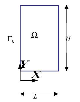
Figure 1.1-a .1-a: Plate scheme
Domain \(\Omega\) dimensions:
\(L=\mathrm{1mm},H=2\pi \text{mm}\)
1.2. Material properties#
The material is elastic with a critical stress and a tenacity chosen arbitrarily:
\(E=10\text{MPa},\nu =\mathrm{0,}{\sigma }_{c}=1.1\text{MPa},{G}_{c}=0.9{\text{N.mm}}^{-1}\)
1.3. Boundary conditions and loads#
The boundary conditions are determined by the analytical solution presented in the next part in such a way that they lead to a crack with a non-constant jump along \({\Gamma }_{0}\). The loading corresponds to a displacement imposed on the edges of the plate: (see [Figure1.3-a]).
\(u=U(x,y)\) |
on \(\Omega /{\Gamma }_{0}\) |
\(u={U}_{0}\delta (y)-(y)\) |
on \({\Gamma }_{0}\) |
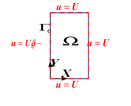
Figure 1.3-a: Load Diagram
The values \(U,{U}_{0}\) and \(\delta\) are set when constructing the reference solution in the next part.