4. Modeling A#
4.1. Characteristics of modeling#
Elastic calculation of a quarter of the plate on a plane stress model (C_PLAN). Charging is defined in § 1.2. We charge up to \(p\mathrm{=}10\mathit{MPa}\).
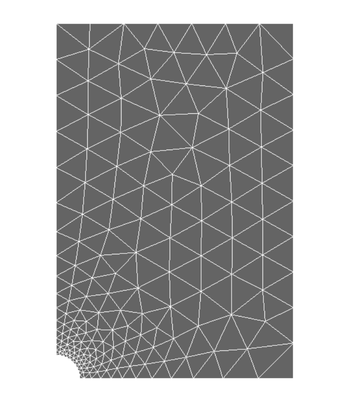
4.2. Characteristics of the mesh#
A quadratic mesh is used.
4.3. Elastic calculation with STAT_NON_LINE#
The aim is to carry out the elastic calculation by generating the AsterStudy command file using the Salome-Meca platform. Modeling is C_PLAN. You should get the same results as using the MECA_STATIQUE command.
4.3.1. Carrying out the calculation#
Start the AsterStudy module.
Then in the left column, click on the Case View tab.
We define the command file for the calculation case (right click on CurrentCase and choose Add Stage).
Note: Add orders using the Commands menu → Show All.
The main steps for creating and launching the calculation case are as follows:
Read the mesh in MED format: Command LIRE_MAILLAGE.
Orient the normal of the edge on which the traction load will be applied: Category Mesh/Command MODI_MAILLAGE/ORIE_PEAU_2D by assigning the top group in GROUP_MA. We keep the same mesh name when using reuse.
Define the finite elements used: Command AFFE_MODELE to assign the MECANIQUE phenomenon and 2D plane stress modeling (C_PLAN) to all elements.
Define material: Command DEFI_MATERIAU .Choose ELAS and enter values for Young’s modulus and Poisson’s ratio.
Assign material to all elements: Command AFFE_MATERIAU.
Assign conditions to kinematic boundaries: Command AFFE_CHAR_CINE/MECA_IMPO for symmetry on the quarter plate (the left and bottom groups).
Affect the load: Command AFFE_CHAR_MECA/FORCE_CONTOUR for the force distributed over the top of the plate. The easiest way is to define a unit load (FY=1.0), which will then be multiplied by a ramp function over time.
Create a linear ramp function \(f=t\) to multiply the unit mechanical load: Command DEFI_FONCTION. For example, it varies between \((\mathrm{0.,}0.)\) and \((\mathrm{1000.,}1000.)\)
Create time discretization using commands DEFI_LIST_REEL and DEFI_LIST_INST. For example, you can determine the end of time at 10s to match the load to \(10\mathit{MPa}\).
Calculate elastic evolution: Command STAT_NON_LINE. We put COMPORTEMENT/RELATION =” ELAS “, the list of times defined previously in INCREMENT, the materials in CHAM_MATER, MODELE and also the boundary conditions and loading (CHARGE + FONC_MULT) in EXCIT.
To launch the calculation case, in the left column, click on the History View tab.
4.3.2. Post-treatments of the results with Aster_Study#
For a non-linear calculation, the STAT_NON_LINEsort command has three fields as standard (depending on the ARCHIVAGE keyword options):
The field of movements at nodes DEPL;
The stress field at Gauss SIEF_ELGA points;
The field of internal variables Gauss points VARI_ELGA.
For post-processing, we also propose to calculate using CALC_CHAMP with reuse:
The node constraint field (SIGM_NOEU) by the CONTRAINTE option.
The equivalent constraints (Von Mises, Tresca, etc.) at the Gauss points, SIEQ_ELGA by option CRITERES.
We suggest printing the results in MED format with IMPR_RESU in order to visualize them in Results orParavis.
Several more advanced post-treatments are then proposed (optional):
Stress extraction SIYYen function of vertical displacement * DYpour the point \(G\) :
Extract the vertical displacement DYau point \(G\): command RECU_FONCTION using the result, and choosing the field DEPLetla component DY.
Extract the constraint SIYYau point \(G\): command RECU_FONCTION using the result, and choosing field SIGM_NOEU and component SIYY.
Print function \(\mathit{SIYY}=f(\mathit{DY})\): Command IMPR_FONCTION in the format XMGRACE (keyword COURBE → FONC_Xet FONC_Y).
Stress extraction SIYY on the lower edge \(\mathit{BD}\) :
Calculate the constraint field by elements at the nodes (SIGM_ELNO): command CALC_CHAMP/CONTRAINTE.
Extract a constraint table SIYYaux from certain points on the \(\mathit{BD}\) edge: command MACR_LIGN_COUPE allows you to extract from a table the components of a field along a given path (keyword LIGN_COUPE). Apply the command to the component SIYYdu field SIGM_ELNO, to the 10 points on the path \(\mathit{BD}\) (giving the coordinates of the points \(B\) and \(D\)).
Print a curve from a table: command IMPR_TABLE to print in XMGRACEla format previous table by filtering on the last moment (for example, FILTRE/NOM_PARA = “INST”, VALE = 10). The X and Y axis parameters of the curve are defined by NOM_PARA: curvilinear abscissa (ABSC_CURV) and constraint (SIYY).
Extraction of constraints on the edge of the hole*:math:`mathit{AB}`*: *
Extract the \({\mathrm{\sigma }}_{\mathrm{\theta }\mathrm{\theta }}\) constraint along the edge of the hole: command MACR_LIGN_COUPE. In the keyword LIGN_COUPE, we specify TYPE = ARC and the coordinate POLAIRE. Define 10 points on the edge of the hole by giving the coordinates of the starting point \(B\) and the center \(O\). At the last moment INST = 10 is filtered and a table is thus produced.
**Note: in the reference* POLAIRE in 2D, The meaning of the components is: * DXrayon \(r\) , * DYangle \(\mathrm{\theta }\). **So* So for for \({\sigma }_{\theta \theta }\) for we have NOM_CMP = SIYY.
Extract the \({\mathrm{\sigma }}_{\mathrm{\theta }\mathrm{\theta }}=f(s)\) function with the curvilinear abscissa \(s=\mathrm{\theta }R\) (\(s\in [\mathrm{0,}R\mathrm{\pi }/2]\)): command RECU_FONCTION. Define PARA_X with the curvilinear abscissa (ABSC_CURV) and PARA_Y with \({\sigma }_{\theta \theta }\) (SIYY).
In elasticity, we can compare this numerical result with the analytical reference (equation).
You can create the analytical formula:command FORMULE. It depends on the curvilinear coordinate \(S\) (NOM_PARA =”S”/VALE =”p* (1.+2. *cos (2).*S/R)) “with \(p\mathrm{=}\mathrm{10MPa}\) and \(R\mathrm{=}\mathrm{10mm}\)).
Create a list of the real values of \(S\) from 0 to \({s}_{\text{max}}=\mathrm{\pi }R/2\): Command DEFI_LIST_REEL.
Interpolation of the formula from the list in \(S\): command CALC_FONC_INTERP.
Command IMPR_FONCTION to print curves of two functions in XMGRACEles format: the one from the numerical result \({\sigma }_{\theta \theta }\mathrm{=}f(s)\) and the one from the analytical formula.
Extraction of the resultant force vertical*at the top of the plate according to vertical displacement:*
Calculate option FORC_NODA with the CALC_CHAMP/FORCE command.
Extract the vertical displacement at point \(G\): command RECU_FONCTION using the result, and choosing field DEPL, DY component.
Extracting vertical resultant force on the top edge of the plate: command MACR_LIGN_COUPE .Choose RESULTATet NOM_CHAM = FORC_NODA. In the LIGN_COUPE keyword, we define points on which we want to calculate the results: give the coordinates of \(G\) and \(F\), the number of points, and RESULTANTE = dy. We then produce a table.
Extract the function from the vertical resultant according to time \({\mathit{Resultante}}_{\mathit{DY}}=f(t)\): command RECU_FONCTION.
Print function \({\mathit{Resultante}}_{\mathit{DY}}=f(\mathit{DY})\): command IMPR_FONCTION in XMGRACE format.
4.4. Tested sizes and results#
We test the value of the stress components for loading \(\mathrm{10MPa}\):
Component |
Reference Type |
Value |
Tolerance |
SIGM_NOEU — \(\mathit{SIYY}\) in \(B\) |
|
|
|
SIGM_NOEU — \(\mathit{SIXX}\) in \(A\) |
|
|
|