3. Modeling A#
The proposed shell modeling is Q4GG. Steel cables are modelled by BARRE elements.
The time step used for the calculations is \(\Delta t\mathrm{=}0.1\mathit{\mu s}\), it respects the stability condition (condition CFL).
3.1. Tested sizes and results#
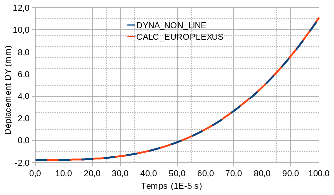
We test the \(\mathit{DY}\) component of the movement at node \({N}_{\mathit{ref}}^{\mathit{cyl}}\) at three different times.
Node |
Component |
Instant (ms) |
Reference Value (m) |
Tolerance (%) |
\({N}_{\mathit{ref}}^{\mathit{cyl}}\) |
|
0 |
|
|
\({N}_{\mathit{ref}}^{\mathit{cyl}}\) |
|
0.5 |
|
|
\({N}_{\mathit{ref}}^{\mathit{cyl}}\) |
|
1 |
|
|
We test the value of two components of the generalized forces \(\mathit{Nxx}\) and \(\mathit{Nyy}\), in the cell \({M}_{\mathit{ref}}^{\mathit{cyl}}\) at three different times.
Mesh |
Component |
Instant (ms) |
Reference Value (N) |
Tolerance (%) |
\({M}_{\mathit{ref}}^{\mathit{cyl}}\) |
|
0 |
|
|
\({M}_{\mathit{ref}}^{\mathit{cyl}}\) |
|
0.5 |
|
|
\({M}_{\mathit{ref}}^{\mathit{cyl}}\) |
|
1 |
|
|
Mesh |
Component |
Instant (ms) |
Reference Value (N) |
Tolerance (%) |
\({M}_{\mathit{ref}}^{\mathit{cyl}}\) |
|
0 |
|
|
\({M}_{\mathit{ref}}^{\mathit{cyl}}\) |
|
0.5 |
|
|
\({M}_{\mathit{ref}}^{\mathit{cyl}}\) |
|
1 |
|
|
The value of the normal force is tested in element \({\mathit{EL}}_{\mathit{ref}}^{\mathit{câb}}\) at three different times.
Mesh |
Component |
Instant (ms) |
Reference Value (N) |
Tolerance (%) |
\({\mathit{EL}}_{\mathit{ref}}^{\mathit{câb}}\) |
|
0 |
|
|
\({\mathit{EL}}_{\mathit{ref}}^{\mathit{câb}}\) |
|
0.5 |
|
|
\({\mathit{EL}}_{\mathit{ref}}^{\mathit{câb}}\) |
|
1 |
|
|
The graph below shows the evolution of the displacement of the reference point obtained either with the DYNA_NON_LINE command or with CALC_EUROPLEXUS.