4. B modeling#
4.1. Characteristics of modeling#
For this modeling, two mobile hardware points are considered according to the following diagram:
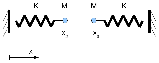
The system is perfectly symmetric. The same formulation as modeling A is obtained if normal shock rigidities equal to half of the rigidities chosen for modeling A.
Indeed, if we note: \({x}_{2}=-{x}_{3}=x\)
The reaction force \({F}_{\mathrm{ext}}\) is in the following form:
During the first phase: \({F}_{\mathrm{ext}}=-{K}_{1}({x}_{2}-{x}_{3})=-2{K}_{1}x\)
During the second phase: \({F}_{\mathrm{ext}}=-{F}_{\mathrm{seuil}}\)
During the third phase: \({F}_{\mathrm{ext}}=-{K}_{2}({x}_{2}-{x}_{3}-2{d}_{p})=-2{K}_{2}(x-{d}_{p})\)
During the fourth phase: \({F}_{\mathrm{ext}}=0\)
We model the problem with an obstacle like BI_PLAN_Y.
At the initial instant, the two hardware points are in contact with an initial speed equal to \(2m\mathrm{/}s\).
The quantities obtained following buckling due to shock are evaluated using the keyword FLAMBAGE of the DYNA_VIBRA operator, with the time diagrams EULER and ADAPT_ORDRE2.
With the adaptive time diagram ADAPT_ORDRE2, we define (in seconds):
the initial time step: PAS = 0.001,
the maximum value of the time step: PAS_MAXI = 0.005.
4.2. Characteristics of the mesh#
Number of knots: 4
Number of stitches: 2 SEG2
4.3. Tested sizes and results#
The values of the quantities related to buckling behavior during the shock are tested.
Identification |
Reference |
T reference type |
Precision |
\({t}_{\mathrm{fl}}\) |
|
“ANALYTIQUE” |
0.01% |
\({d}_{p}\) |
3 m |
“ANALYTIQUE” |
0.01% |
\(x({t}_{0})=x(\frac{\pi }{6}+2\sqrt{3}+\frac{\pi +6}{\sqrt{2}})\) |
0m |
“ANALYTIQUE” |
1.e-4m |