5. C modeling#
This modeling is exactly the same as modeling A. The only difference is in the mesh: the HEXA8 of mesh A are cut in TETRA4.
5.1. Characteristics of modeling#
We use the 3D modeling of the THERMIQUE phenomenon.
5.2. Characteristics of the mesh#
The mesh includes 30 TETRA4 meshes.
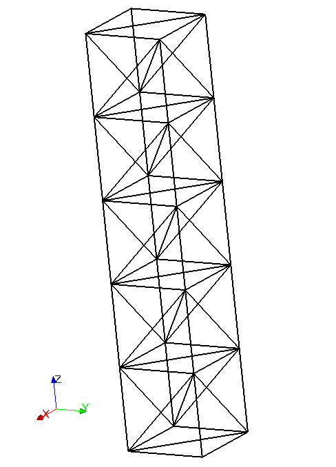
Figure 5.2-1: C mesh
5.3. Tested sizes and results#
We first test the values of the classical degrees of freedom TEMP and Heaviside H1 of the temperature field at the output of the THER_LINEAIRE operator, at the nodes located just below (4 knots) and above the interface (4 knots).
Identification |
Reference type |
Reference value |
Tolerance |
|
All nodes located just above the interface - \(\mathit{TEMP}\) |
“ANALYTIQUE” |
20 |
|
|
All nodes just below the interface - \(\mathit{TEMP}\) |
“ANALYTIQUE” |
“” |
10 |
|
All nodes located just below/above the interface - \(\mathit{H1}\) |
“ANALYTIQUE” |
5 |
|
We then test the value of the degree of freedom TEMP of the temperature field at the outlet of POST_CHAM_XFEM, at the nodes located just below and above the interface.
Identification |
Reference type |
Reference value |
Tolerance |
|
All nodes just below the interface - \(\mathit{TEMP}\) |
“ANALYTIQUE” |
“” |
10 |
|
All nodes located just above the interface - \(\mathit{TEMP}\) |
“ANALYTIQUE” |
20 |
|
Finally, we test the value of the TEMP component of the TEMP_ELGA field on the Gauss points located below and above the interface (cf. note page 6).
Identification |
Reference type |
Reference value |
Tolerance |
|
On the Gauss points below the interface - \(\mathit{TEMP}\) |
“ANALYTIQUE” |
“” |
10 |
|
On the Gauss points above the interface - \(\mathit{TEMP}\) |
“ANALYTIQUE” |
“” |
20 |
|