5. C modeling: X- FEM 3D modeling#
5.1. Characteristics of modeling#
In this modeling, the crack is not meshed (case X- FEM) and the structure is modeled in 3D. Only a quarter of the structure is modelled, for reasons of symmetry.
The crack is represented by level sets:
\(\mathit{lsn}\mathrm{=}\sqrt{{x}^{2}+{(y\mathrm{-}R)}^{2}+{z}^{2}}\mathrm{-}R\)
\(\mathit{lst}\mathrm{=}\sqrt{{x}^{2}+{(y\mathrm{-}{y}_{h})}^{2}+{z}^{2}}\mathrm{-}R\text{'}\)
with \({y}_{h}\mathrm{=}R\mathrm{-}\frac{R}{\mathrm{cos}(\alpha )}\) and \(R\text{'}\mathrm{=}R\mathrm{tan}(\alpha )\)
Note:
In 3 D , there is an arbitrary choice of orientation of the local base at the bottom of the crack. Depending on the orientation of this base, the sign of \({K}_{\mathit{II}}\) and \({K}_{\mathit{III}}\) will be different (because it is linked to the base). But this has no influence on the physical result (angle of possible bifurcation of the crack expressed in the global coordinate system). Here, to find \({K}_{\mathit{II}}>0\) as in the reference solution, you must define the normal level set as the opposite of the formula above. In this modeling, we will finally remember \(\mathit{lsn}\mathrm{=}\mathrm{-}\sqrt{{x}^{2}+{(y\mathrm{-}R)}^{2}+{z}^{2}}+R\). It remains a convention and does not change the physical result!
In 2 D*, the sign of the normal level set does not affect the sign of* \({K}_{\mathit{II}}\) because there is no choice x*to define the local base.*
5.2. Characteristics of the mesh#
The initial healthy mesh is relatively coarse: 2508 knots and 11945 TETRA4. The mesh size is \({h}_{0}\mathrm{=}1m\). A successive refinement procedure is used to arrive at a target size that is substantially identical to that of modeling A, i.e. \({h}_{c}\mathrm{=}\mathrm{0,025}m\). To do this, we call Lobster iteratively. After refinement, the mesh size near the bottom of the crack is \(h\mathrm{=}\mathrm{0,015625}m\). All the meshes are refined in a disk with radius \(5h\) around the bottom of the crack.
Number of knots: 18166
Number of meshes and type: 103079 TETRA4
The characteristic length of an element near the crack bottom is 0.0156 m.
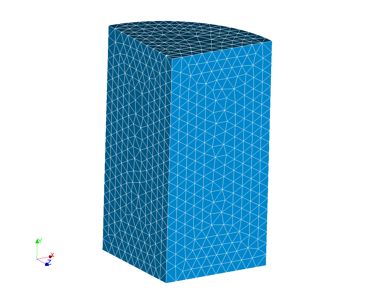
Figure 5.2-1: initial mesh
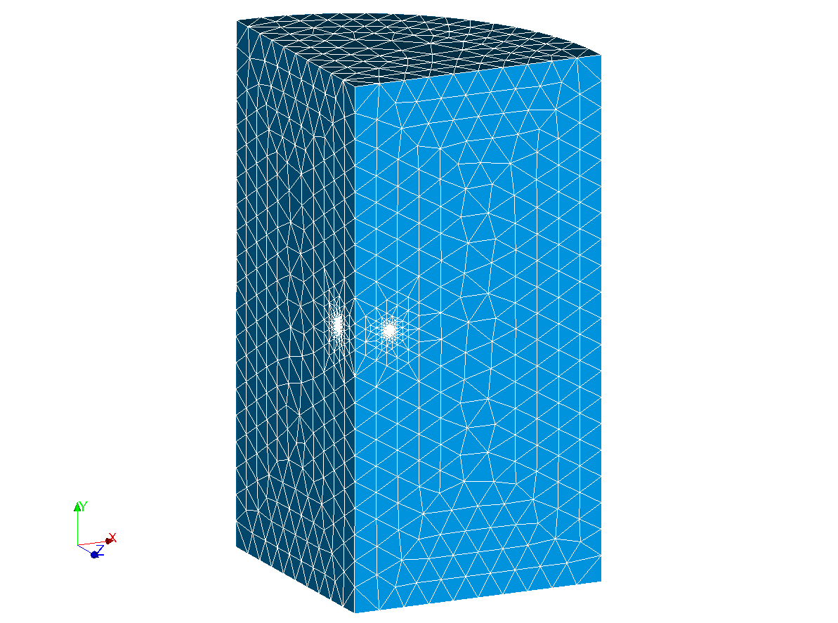
Figure 5.2-2: refined mesh
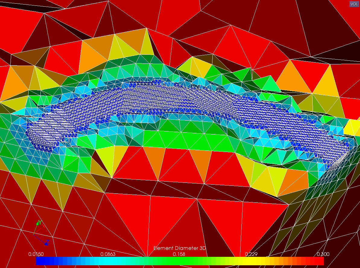
Figure 5.2-3: Size map on a section of the refined mesh
5.3. Boundary conditions and loads#
A surface tensile force is applied on the upper, lower and outer faces;
Symmetry conditions on the lateral faces are applied;
The rigid mode of movement along the \(\mathit{Oy}\) axis is blocked by blocking a node along this axis.
5.4. Tested sizes and results#
The choice of numerical parameters for post-processing SIFs is identical to that made for modeling A: \({R}_{\text{inf}}\mathrm{=}2h\) and \({R}_{\text{sup}}\mathrm{=}5h\).
5.4.1. Values from CALC_G_XFEM#
The values are in \(\mathit{Pa}\mathrm{.}\sqrt{m}\).
Identification |
Reference type |
Reference value |
Tolerance |
\(\mathit{max}({K}_{I})\) |
“ANALYTIQUE” |
1.177 106 |
|
\(\mathit{min}({K}_{I})\) |
“ANALYTIQUE” |
1.177 106 |
|
\(\mathit{max}({K}_{\mathit{II}})\) |
“ANALYTIQUE” |
0.3153 106 |
|
\(\mathit{min}({K}_{\mathit{II}})\) |
“ANALYTIQUE” |
0.3153 106 |
|
5.4.2. Values from POST_K1_K2_K3#
The values are in \(\mathit{Pa}\mathrm{.}\sqrt{m}\).
Identification |
Reference type |
Reference value |
Tolerance |
\(\mathit{max}({K}_{I})\) |
“ANALYTIQUE” |
1.177 106 |
|
\(\mathit{min}({K}_{I})\) |
“ANALYTIQUE” |
1.177 106 |
|
\(\mathit{max}({K}_{\mathit{II}})\) |
“ANALYTIQUE” |
0.3153 106 |
|
\(\mathit{min}({K}_{\mathit{II}})\) |
“ANALYTIQUE” |
0.3153 106 |
|
5.4.3. Comments#
By further refining the mesh, we can reduce the error, but the calculation time becomes incompatible with that of a test case.
Figure 5.4.3-1: comparison of the K between the different methods