4. Modeling B: Modeling X- FEM 2d-AXI#
4.1. Characteristics of modeling#
In this modeling, the crack is not meshed (case X- FEM) and the structure is modeled using 2D-axisymmetry.
The crack is represented by level sets:
\(\mathit{lsn}=\sqrt{{x}^{2}+{(y-R)}^{2}}-R\)
\(\mathit{lst}=\sqrt{{x}^{2}+{(y-{y}_{h})}^{2}}-R\text{'}\)
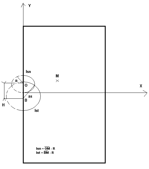
Figure 4.1-1: Level sets with \({y}_{h}=R-\frac{R}{\mathrm{cos}(\alpha )}\) and \(R\text{'}=R\mathrm{tan}(\alpha )\)
4.2. Characteristics of the mesh#
The initial healthy mesh is relatively coarse: 252 knots and 442 TRIA3. The mesh size is \({h}_{0}=1m\). A successive refinement procedure is used to arrive at a target size corresponding to half the mesh size of modeling A, i.e. \({h}_{c}=\mathrm{0,0125}m\). Indeed, modeling A uses quadratic elements, so finer linear elements are needed to obtain equivalent precision. To do this, we call Lobster iteratively. After refinement, the size of the meshes close to the bottom of the crack is \(h=\mathrm{0,0078125}m\). All the meshes are refined in a disk with radius \(5h\) around the bottom of the crack.

Figure 4.2-1: initial healthy mesh
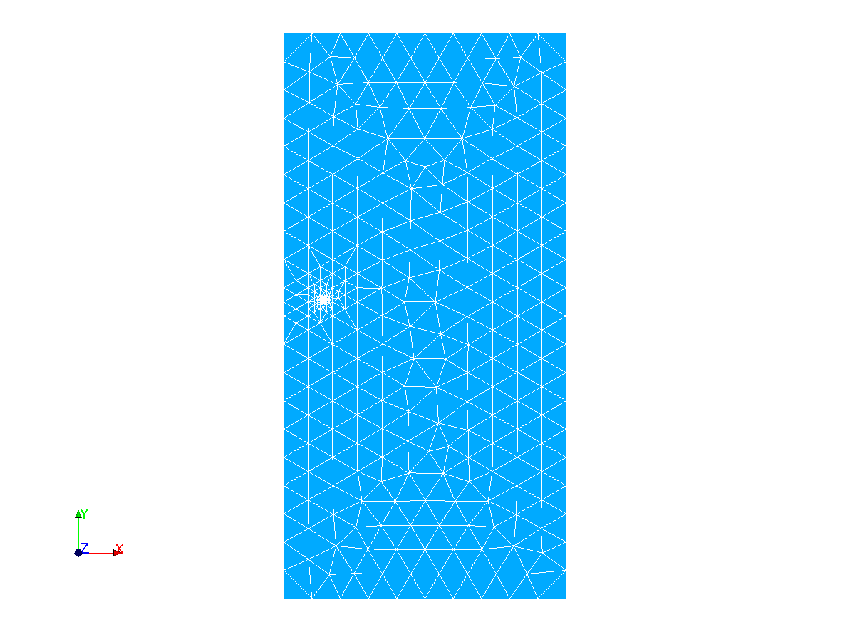
Figure 4.2-2: refined healthy mesh
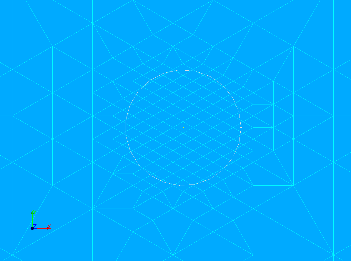
Figure 4.2-3: zoom on the refined part (the disk of the refinement zone is also shown)
Number of knots: 722
Number of meshes and type: 1442 TRIA3
The characteristic length of an element near the crack bottom is 0.0078 m.
This size is smaller than the target size (for reasons of integer division by 2 during refinement).
4.3. Boundary conditions and loads#
A surface tensile force is applied to the upper, lower and right sides;
The movements following \(\mathit{Ox}\) of the nodes of the axis of rotation are blocked, as recommended for axisymmetric models;
The rigid mode of movement along the \(\mathit{Oy}\) axis is blocked by blocking a node along this axis.
4.4. Tested sizes and results#
The choice of numerical parameters for post-processing SIFs is identical to that made for modeling A: \({R}_{\text{inf}}=\mathrm{2h}\) and \({R}_{\text{sup}}=\mathrm{5h}\), but \(h\) here is worth less than half of the \(h\) of modeling A.
4.4.1. Values from CALC_G_XFEM#
The values are in \(\mathit{Pa}\mathrm{.}\sqrt{m}\).
Identification |
Reference Type |
Reference Value |
% Tolerance |
\({K}_{I}\) |
“ANALYTIQUE” |
1,177 106 |
|
\({K}_{\mathit{II}}\) |
“ANALYTIQUE” |
0.3153 106 |
|
4.4.2. Values from POST_K1_K2_K3#
The values are in \(\mathit{Pa}\mathrm{.}\sqrt{m}\).
Identification |
Reference Type |
Reference Value |
% Tolerance |
\({K}_{I}\) |
“ANALYTIQUE” |
1,177 106 |
|
\({K}_{\mathit{II}}\) |
“ANALYTIQUE” |
0.3153 106 |
|