2. Benchmark solution#
2.1. Calculation method#
For both loading cases, the reinforcement is calculated using the Capra-Maury method (command CALC_FERRAILLAGE called by the command COMBINAISON_FERRAILLAGE).
2.2. Reference quantities and results#
This system is equivalent to a built-in beam loaded with bending at the free end:
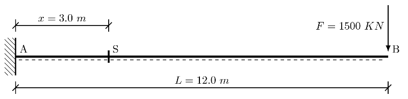
Figure 3. Representation of an embedded and flexurally loaded beam
A first estimate of movements and efforts can therefore be obtained with Euler-Bernoulli modeling:
Arrow: \(f=\frac{1}{3}\cdot \frac{F{L}^{3}}{EI}\), such as \(\mathit{EI}=30000\cdot {10}^{6}\times (\frac{{\mathrm{3,0}}^{3}\cdot \mathrm{0,3}}{12})=\mathrm{20,25}\cdot {10}^{9}N{m}^{2}\)
Either:
\(f=\frac{1}{3}\cdot (\frac{{\mathrm{12,0}}^{3}}{\mathrm{20,25}\cdot {10}^{9}})\times F=\mathrm{2,84}\cdot {10}^{-8}\times F\)
Shear: \(V=F\)
Bending moment at embedment: \(M=F\times L\)
Thus, the following results are obtained:
sHearld1 |
sHearld2 |
sHearld3 |
|
F |
\(-\mathrm{1,5}\cdot {10}^{6}N\) |
|
|
V |
\(\mathrm{1,5}\cdot {10}^{6}N\) |
|
|
M |
\(-\mathrm{1,8}\cdot {10}^{7}\mathit{Nm}\) |
|
|
f |
\(\mathrm{42,6}\mathit{mm}\) |
|
|
For cases with axial loading (tractLD and ComPld), the shrinkage/elongation of the beam is obtained analytically as follows:
Arrow: \(\mathrm{\Delta }L=\frac{F\cdot L}{E\cdot S}\), such as \(\mathit{ES}=30000\cdot {10}^{6}\times 3\times \mathrm{0,3}=\mathrm{2,7}\cdot {10}^{10}N\)
Either:
\(\mathrm{\Delta }L=\mathrm{4,44}\cdot {10}^{-10}\times F\)
Normal force using the beam: \(N=-F\) (positive normal force under compression).
Thus, the following results are obtained:
tractLD1 |
tractLD2 |
tractLD2 |
tractLD3 |
compLD1 |
compLD2 |
|
F |
\(+\mathrm{1,0}\cdot {10}^{6}N\) |
|
|
|
|
|
N |
\(-\mathrm{1,0}\cdot {10}^{6}N\) |
|
|
|
|
|
f |
\(+\mathrm{0,44}\mathit{mm}\) |
|
|
|
|
For the calculation of reinforcement according to the Capra Maury method, analog resonance is applied to the simple analytical cases proposed in the test case relating to this method, namely ssls134.
2.3. Uncertainty about the solution#
The solution is analytical. The differences between the analytical solution and the reference solution in non-regression are due to the fact that the beam is quite slightly slender (high \(H/L\) ratio) and we are therefore approaching the limits of the Euler-Bernoulli model.