10. H modeling#
10.1. Characteristics of modeling#
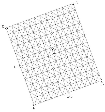
COQUE_3D triangular shell element
The plate model associated with modeling \(E\) is rotated 20 degrees according to the alpha nautical angle and 30 degrees according to beta. The cell numbering is the same as in modeling \(E\).
Boundary conditions:
LIAISON_OBLIQUE |
(GROUP_NO: AB, ANGL_NAUT =( 20.,30.,0.) , EX: 0. , DZ: 0. , DRY :0.) |
(GROUP_NO: BC, ANGL_NAUT =( 20.,30.,0.) , BY: 0. , DZ: 0. , DRX :0.) |
(GROUP_NO: CD, ANGL_NAUT =( 20.,30.,0.) , EX: 0. , DZ: 0. , DRY :0.) |
(GROUP_NO: DA, ANGL_NAUT =( 20.,30.,0.) , BY: 0. , DZ: 0. , DRX :0.) |
(GROUP_NO: O, ANGL_NAUT =( 20.,30.,0.) , EX: 0. , BY: 0. , DRX :0. , DRY :0. , DRZ :0.) |
FORCE_ARETE |
(GROUP_NO: AB MY:0.) |
(GROUP_NO: BC MX:0.) |
(GROUP_NO: CDMY:0.) |
(GROUP_NO: BY MAX:0.) |
10.2. Characteristics of the mesh#
Number of knots: 626
Number of meshes and type: 288 TRIA6
10.3. Tested sizes and results#
Identification |
|
Point O \((\mathit{M134})\) |
|
Constrains |
\({\sigma }_{\mathit{xx}}\), \({\sigma }_{\mathit{yy}}\),, \({\sigma }_{\mathit{xy}}\),,, \({\sigma }_{\mathit{xz}}\), \({\sigma }_{\mathit{yz}}\) on lower, middle, and upper sheets |
Displacement |
\(\mathit{DZ}\) |
Point B1 \((\mathit{M122})\) |
|
Constraints |
\({\sigma }_{\mathit{xx}}\), \({\sigma }_{\mathit{yy}}\), \({\sigma }_{\mathit{xy}}\), \({\sigma }_{\mathit{xz}}\), \({\sigma }_{\mathit{yz}}\) on lower, middle and upper sheets |
Identification |
||
Point O |
\((\mathit{M134})\) |
\({N}_{\mathit{xx}}\), \({N}_{\mathit{yy}}\), \({N}_{\mathit{xy}}\), \({M}_{\mathit{xx}}\), \({M}_{\mathit{yy}}\),, \({M}_{\mathit{xy}}\), \({T}_{x}\), \({T}_{y}\) |
\((\mathit{M158})\) |
|
|
\((\mathit{M132})\) |
|
|
\((\mathit{M156})\) |
|
|
Point A |
\((\mathit{M1})\) |
\({N}_{\mathit{xx}}\), \({N}_{\mathit{yy}}\), \({N}_{\mathit{xy}}\), \({M}_{\mathit{xx}}\), \({M}_{\mathit{yy}}\),, \({M}_{\mathit{xy}}\), \({T}_{x}\), \({T}_{y}\) |
Point B |
\((\mathit{M266})\) |
\({N}_{\mathit{xx}}\), \({N}_{\mathit{yy}}\), \({N}_{\mathit{xy}}\), \({M}_{\mathit{xx}}\), \({M}_{\mathit{yy}}\),, \({M}_{\mathit{xy}}\), \({T}_{x}\), \({T}_{y}\) |
Identification |
||
Point C |
\((\mathit{M288})\) |
\({N}_{\mathit{xx}}\), \({N}_{\mathit{yy}}\), \({N}_{\mathit{xy}}\), \({M}_{\mathit{xx}}\), \({M}_{\mathit{yy}}\),, \({M}_{\mathit{xy}}\), \({T}_{x}\), \({T}_{y}\) |
Point D |
\((\mathit{M23})\) |
\({N}_{\mathit{xx}}\), \({N}_{\mathit{yy}}\), \({N}_{\mathit{xy}}\), \({M}_{\mathit{xx}}\), \({M}_{\mathit{yy}}\),, \({M}_{\mathit{xy}}\), \({T}_{x}\), \({T}_{y}\) |
Identification |
||
Point B1 |
\((\mathit{M122})\) |
\({N}_{\mathit{xx}}\), \({N}_{\mathit{yy}}\), \({N}_{\mathit{xy}}\), \({M}_{\mathit{xx}}\), \({M}_{\mathit{yy}}\),, \({M}_{\mathit{xy}}\), \({T}_{x}\), \({T}_{y}\) |
\((\mathit{M146})\) |
\({N}_{\mathit{xx}}\), \({N}_{\mathit{yy}}\), \({N}_{\mathit{xy}}\), \({M}_{\mathit{xx}}\), \({M}_{\mathit{yy}}\),, \({M}_{\mathit{xy}}\), \({T}_{x}\), \({T}_{y}\) |
|
Identification |
||
Point D1 |
\((\mathit{M11})\) |
|
\((\mathit{M14})\) |
\({N}_{\mathit{xx}}\), \({N}_{\mathit{yy}}\), \({N}_{\mathit{xy}}\), \({M}_{\mathit{xx}}\), \({M}_{\mathit{yy}}\),, \({M}_{\mathit{xy}}\), \({T}_{x}\), \({T}_{y}\) |
|
10.4. notes#
The reference value of the displacement at point \(O\) is obtained by projecting the displacement calculated for the modeling E into the rotated coordinate system (the displacement for the modeling E being vertical, the new displacement is a function of the projection of the axis \(Z\)).
In the local coordinate system, the projection of the \(Z\) axis is as follows:
, with
and
On the other hand, the expression for the sine pressure in the rotated coordinate system becomes: