3. B modeling#
3.1. Meshing#
The mesh of the three parts of the pump is provided, as well as its complete mesh. After importing the meshes into SALOME - MECA, we will take the time needed to find the names of the groups needed for the data layout.
The mesh is made of 3S solid elements in DKT plate elements. The plate elements correspond to a thickness of:
\(30\mathit{mm}\) for the tier (“Pal_2D” group)
\(50\mathit{mm}\) for volute (group “Vol_2D”)
\(10\mathit{mm}\) for the pipe (group “Vol_2D”)
3.2. Aster command file#
The main steps of the calculation with Aster are, for each substructure, the usual data processing steps:
Reading the mesh in MED format (LIRE_MAILLAGE (“FORMAT =” MED”)). |
Definition of the finite elements used (AFFE_MODELE). “3D” and “DKT” modeling |
Material definition and assignment (DEFI_MATERIAU and AFFE_MATERIAU). |
Assigning the characteristics of plate elements (AFFE_CARA_ELEM). |
Assigning boundary conditions (AFFE_CHAR_MECA). |
Then the construction of the macro-elements, their assembly, the modal calculation of the assembled structure, the construction of the skeleton, the restoration of the modal calculation on the skeleton and, finally, the impression of the modes:
Creation of substructures (CREA_ELEM_SSD) |
Assembling the substructures (ASSE_ELEM_SSD) |
Modal calculation (CALC_MODES) |
Construction of the global mode visualization skeleton (DEFI_SQUELETTE) |
Restitution on the skeleton (REST_SOUS_STRUC) |
Fashion printing in MED format (IMPR_RESU) |
The aim is to specify the type of substructure to be used when creating substructures. Here we have:
TYPE =” RITZ “
TYPE_MODE =” INTERFACE “
3.3. Results#
The quantities compared are the frequencies of the first 10 natural modes of the pump obtained during the direct calculation carried out on the global mesh with those obtained by substructuring on the pump divided into three parts.
Mode |
Direct modal calculation (Hz) |
Calculation by SSD (Hz) |
1 |
58.32 |
58.43 |
2 |
123.47 |
146.72 |
3 |
155.27 |
185.43 |
4 |
190.57 |
196.71 |
5 |
224.85 |
229.52 |
6 |
230.77 |
236.14 |
7 |
249.22 |
256.57 |
8 |
259.38 |
263.87 |
9 |
261.07 |
275.37 |
10 |
278.07 |
287.58 |
It can be seen that the frequencies calculated by the two methods are quite similar.
We can also verify in SALOME - MECA that this is also the case for modal deformations.
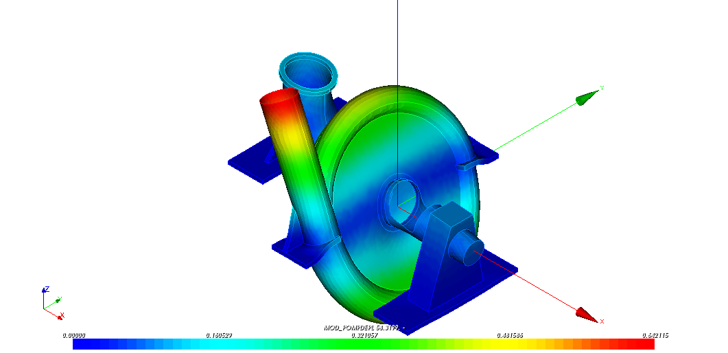
Figure 9: Mode 1 of the direct modal calculation |
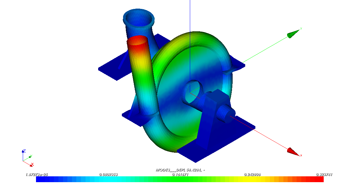
Illustration 10: Mode 1 of the SSD calculation using the interface method |
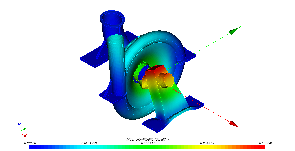
Figure 11: Mode 2 of the direct modal calculation |
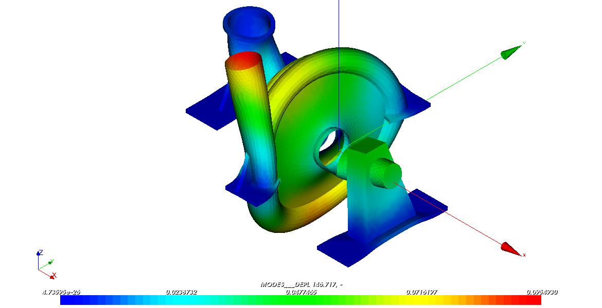
Illustration 12: Mode 2 of the SSD calculation using the interface method |
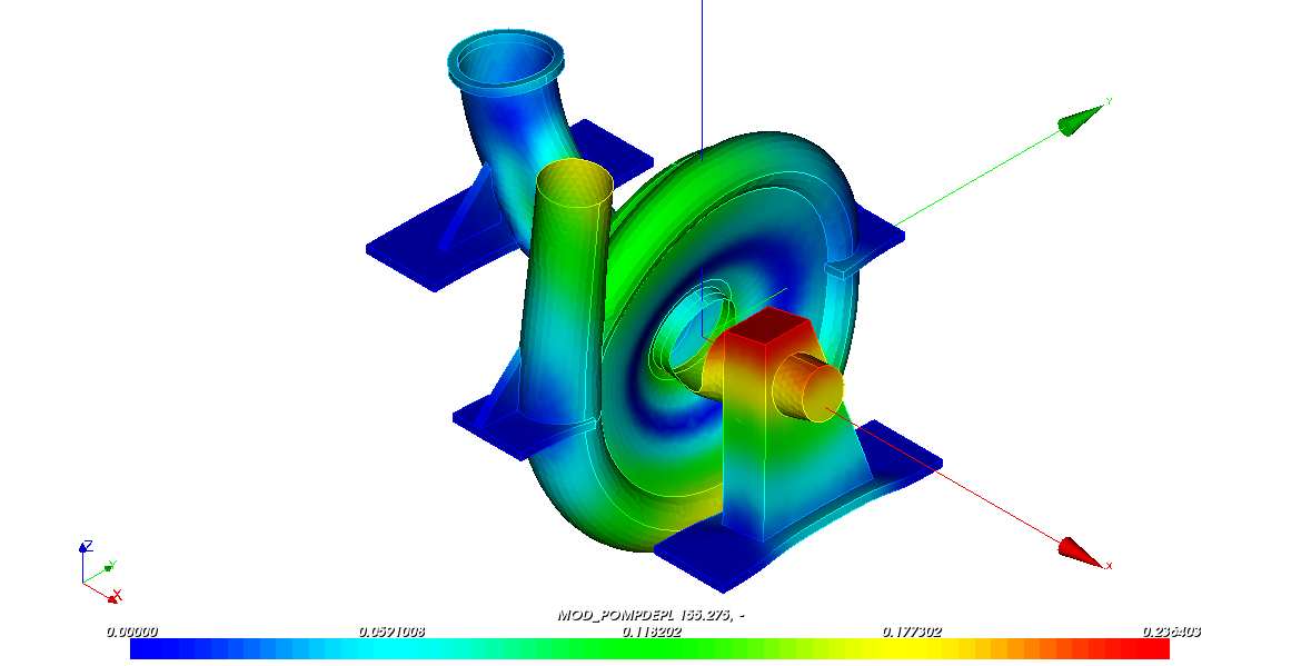
Figure 13: Mode 3 of the direct modal calculation |
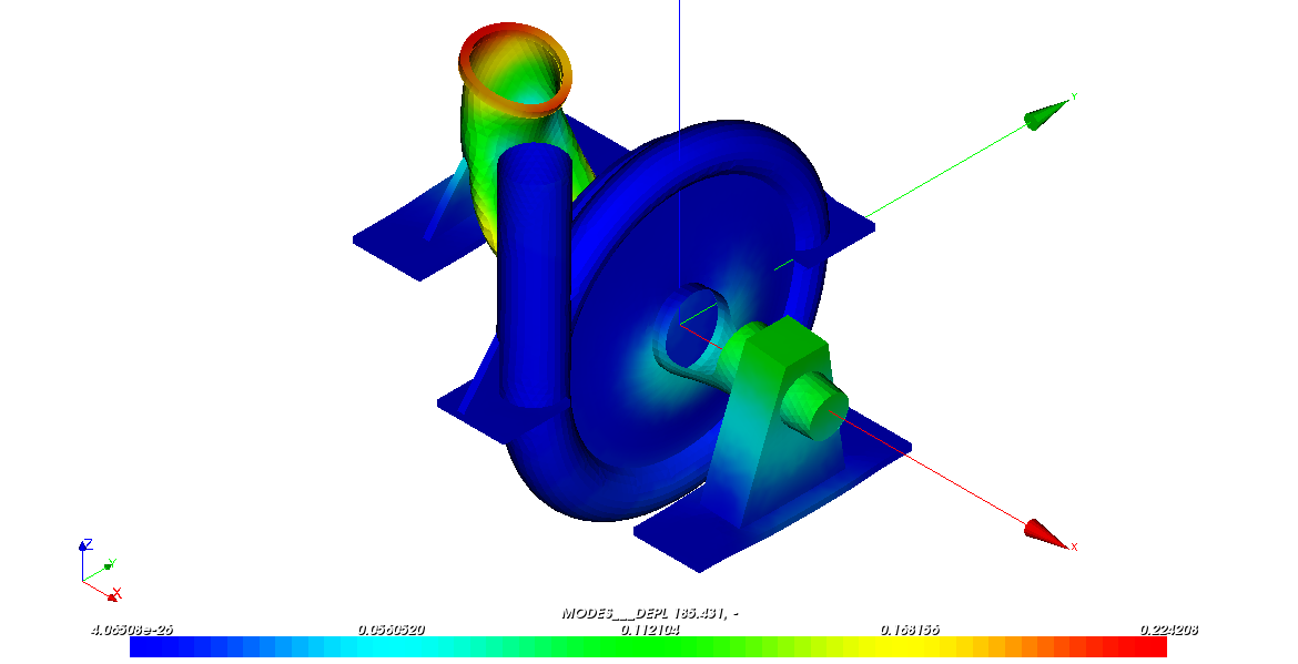
Illustration 14: Mode 3 of the SSD calculation using the interface method |