3. C modeling#
3.1. Problem description#
The objective of this modeling is the use of the macro command CALC_MODES [U4.52.02] with the option “BANDE” divided into several sub-bands. This command allows you to start a succession of real eigenmode calculations.
The following actions are carried out:
Obtaining modes by simultaneous iterations, in specified frequency bands,
Application of a standard, filtering according to a criterion of modal parameter value greater than a certain threshold and finally concatenation of the calculated data structures into a single one.
The modes are calculated by the CALC_MODES [U4.52.02] command with the “BANDE” option and normalized by the NORM_MODE [U4.52.11] command. The calculated modes are filtered and concatenated using the EXTR_MODE [U4.52.12] command.
3.1.1. Objective#
The objective of this modeling is:
To « weigh » the finite element model and to evaluate the number of modes,
To use the macro command CALC_MODES with the option “BANDE” divided into several sub-bands to calculate the natural frequencies.
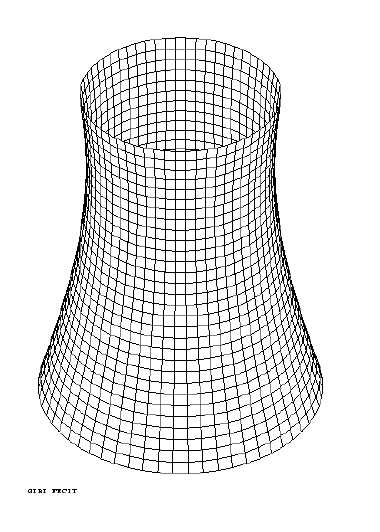
3.1.2. Geometry#
You can retrieve the mesh in the test case directory.
The thickness of the shell is \(e=\mathrm{0,3045}m\)
3.1.3. Material Properties#
The material is linear isotropic elastic:
Young’s module \(E=\mathrm{2,76}\mathrm{.}{10}^{10}N/{m}^{2}\),
Poisson’s ratio \(\nu =\mathrm{0,166}\),
density \(\rho =2244\mathrm{Kg}/{m}^{3}\)
3.1.4. Boundary conditions and loading#
The tower is embedded at its base.
3.2. Characteristics of modeling#
3.2.1. Characteristics of the mesh#
The mesh is composed of 1860 QUAD4 and 1860 knots
The tower is modelled with shell elements DKT
3.2.2. Aster commands#
The main steps of the calculation with*Aster* will be:
Reading the mesh (LIRE_MAILLAGE). |
Definition of the finite elements used (AFFE_MODELE). We will assign modeling DKT to all the elements of the tower. |
Material definition and assignment (DEFI_MATERIAU and AFFE_MATERIAU). |
The mechanical characteristics are identical throughout the structure. |
Assigning shell element characteristics (AFFE_CARA_ELEM). |
The thickness of all the elements is the same. |
Assigning boundary conditions (AFFE_CHAR_MECA). |
Calculation of elementary stiffness matrices (CALC_MATR_ELEM ((OPTION =” RIGI_MECA “)). |
Calculation of elementary mass matrices (CALC_MATR_ELEM ((OPTION =” MASS_MECA “). |
Numbering the unknowns of a system of linear equations (NUME_DDL) |
Assembly of elementary mass and stiffness matrices (ASSE_MATRICE). |
Note: to go faster we can use the macro ASSEMBLAGE to build the matrices!
Question #1:
Weigh the model (POST_ELEM) and assess the number of modes whose frequency is less than \(4\mathrm{Hz}\) (INFO_MODE).
Question #2:
Calculate the natural frequencies and the first associated modes present in the frequency band \(0.\mathrm{Hz}\) to \(4\mathrm{Hz}\) (CALC_MODES)
Normalize with the infinite norm, on all components of physical nodes while requiring the calculation of effective unit masses (NORM_MODE, EXTR_MODE).
Print the proper modes (IMPR_RESU) in MED format for viewing in Salome.
Question #3:
Calculate the natural frequencies by grouping the three operations CALC_MODES, NORM_MODE and EXTR_MODE into one (by cutting into 2 intervals) with CALC_MODES and the option “BANDE” divided into several sub-bands.
Question #4:
Calculate the natural frequencies by grouping the three operations CALC_MODES, NORM_MODE and EXTR_MODE into one (by cutting into 4 intervals) with CALC_MODES and the option “BANDE” divided into several sub-bands.
Question #5:
We achieve the same thing as that asked in question 4 but with the method of LANCZOS.
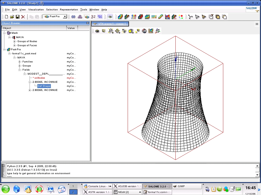
3.3. Help with post-treatment under Salome#
The different steps for visualizing modal deformations with Salomé are as follows:
Start Salome on Linux |
Start the Mesh/New mesh module |
Click on File/Import/ MED file and select the med file containing the mesh |
Start the Post-Pro post-processing module |
Click on File/Import/ MED file and select the med file containing the specific modes to be viewed |
Deploy the Post-Pro line tree completely in the Object Browser in order to see all the movement fields in detail. |
Click on one of the fields and with the right mouse button click on Deformed Shape. (modal distortion is displayed). |
Deploy the line containing the visualized field, then click on Def. Shape and then click on the right mouse button and select Sweeper to animate the deformation. |
3.4. notes#
Best practices: you must first:
Weigh your model with POST_ELEM, |
Evaluating the spectrum with INFO_MODE. |
The CALC_MODES command, with the “BANDE” option divided into several sub-bands, is more economical to search for a large spectrum.
As long as you don’t overcook it, |
It is necessary to verify the agreement of the identified bits of spectrum, |
Saving time can be very important: \(\text{500\%}\), |
You can easily and automatically add other operations to it: normalization, filtering, concatenation of data structures. |
3.5. Tested sizes and results#
Mode |
Frequency in \(\mathrm{Hz}\) |
1 |
|
2 |
|
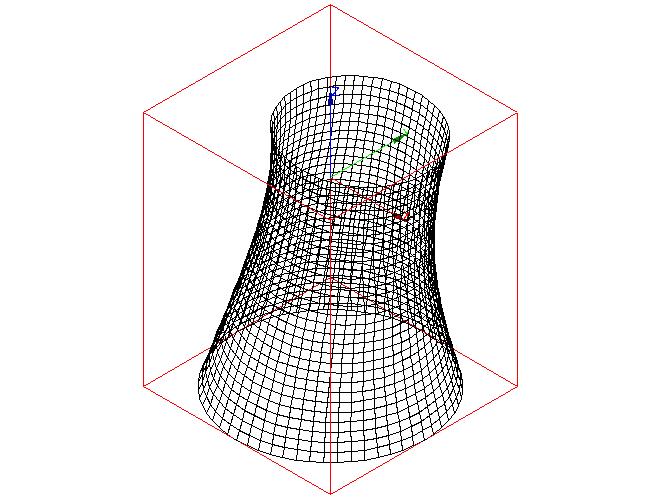
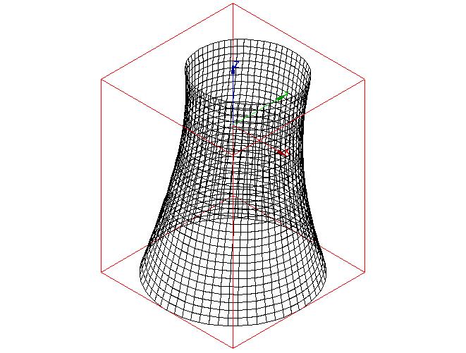
Modal warp ( \(2.80065\mathrm{Hz}\) ) Modal warp ( \(2.80065\mathrm{Hz}\) )