2. B modeling#
2.1. Problem description#
2.1.1. Objective#
The objective of this modeling is to determine for a free free sphere-type structure, (presence of multiple rigid body modes):
Natural frequencies located in a frequency band using the SORENSEN method,
Natural frequencies located in a frequency band using the LANCZOS method with or without rigid mode (OPTION = MODE_RIGIDE),
The 16 smallest natural frequencies with the SORENSEN method
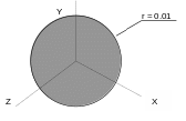
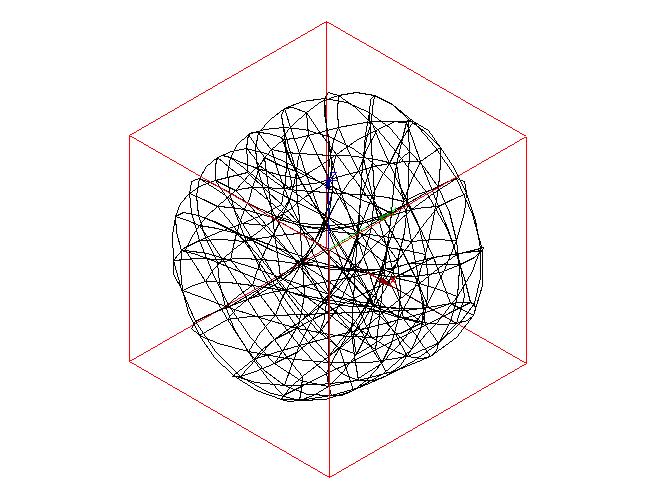
2.1.2. Geometry#
2.1.3. Material properties#
The material is linear isotropic elastic:
Young’s module \(E={10}^{8}N/{m}^{2}\),
Poisson’s ratio \(\nu \mathrm{=}0.3\),
density \(\rho ={10}^{4}\mathrm{kg}/{m}^{3}\)
2.1.4. Boundary conditions and loading#
None
2.2. Characteristics of modeling#
2.2.1. Characteristics of the mesh#
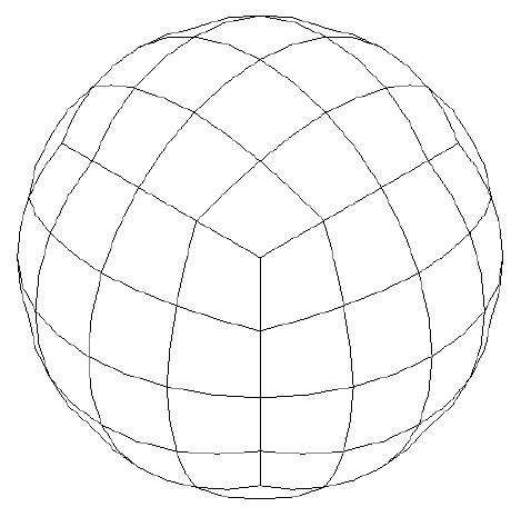
The mesh includes 160 HEXA20 stitches, and 813 knots.
Solid elements (3D) will be used for modeling.
2.2.2. Aster commands#
The main steps of the calculation with*Aster* will be:
Reading the mesh (LIRE_MAILLAGE). |
Definition of the finite elements used (AFFE_MODELE). |
Material definition and assignment (DEFI_MATERIAU and AFFE_MATERIAU). |
The mechanical characteristics are identical throughout the structure. |
Calculation of elementary stiffness matrices (CALC_MATR_ELEM ((OPTION =” RIGI_MECA “)). |
Calculation of elementary mass matrices (CALC_MATR_ELEM ((OPTION =” MASS_MECA “) |
Numbering the unknowns of the system of linear equations (NUME_DDL) |
Assembly of elementary mass and stiffness matrices (ASSE_MATRICE). |
**Note:* to go faster we can use the macro ASSEMBLAGE to build the matrices!
Question #1:
Calculate with the SORENSEN method (under the keyword factor SOLVEUR_MODAL), the frequencies located in the \((0.\mathrm{Hz},2880\mathrm{Hz})\) frequency band as well as the associated modes (CALC_MODES).
If the calculation fails we can extend the frequency band by a slightly negative margin.
Print the proper modes (IMPR_RESU) in MED format for viewing in Salome.
Question #2:
Calculate with the LANCZOS method with or without option MODE_RIGIDE the frequencies located in the \((0.\mathrm{Hz},2880\mathrm{Hz})\) frequency band as well as the associated modes (CALC_MODES).
Question #3:
Calculate with the SORENSEN method the 16 smallest frequencies as well as the associated modes (CALC_MODES). We can use the parameter PREC_SHIFT (under the keyword factor CALC_FREQ) to get around the problem of zero frequencies.
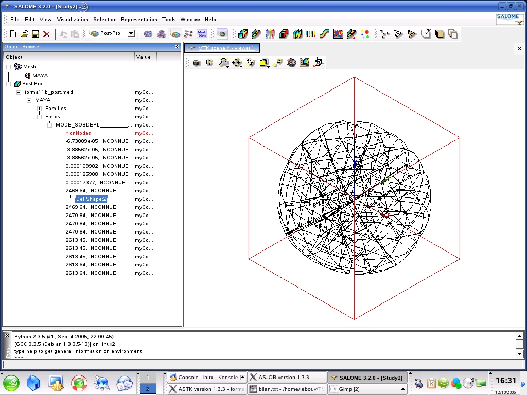
2.3. Help with post-treatment under Salome#
The different steps for visualizing modal deformations with Salomé are as follows:
Start Salome on Linux |
Start the Mesh/New mesh module |
Click on File/Import/ MED file and select the med file containing the mesh |
Start the Post-Pro post-processing module |
Click on File/Import/ MED file and select the med file containing the specific modes to be viewed |
Deploy the Post-Pro line tree completely in the Object Browser in order to see all the movement fields in detail. |
Click on one of the fields and with the right mouse button click on Deformed Shape. (modal distortion is displayed). |
Deploy the line containing the visualized field, then click on Def. Shape and then click on the right mouse button and select Sweeper to animate the deformation. |
2.4. notes#
The factorization of the \({(K-\sigma \text{})}^{-1}={\mathrm{LDL}}^{T}\) shifted matrices governed by the parameterization: NMAX_ITER_SHIFT, SOLVEUR/NPREC [U4.50.01] and PREC_SHIFT, can only be done if they are regular.
This is often a problem when the magnitude of the terms in \(K\) is greater than the magnitude of the terms in \(M\) and \(\sigma\) is a good approximate eigenvalue. The operator’s policy is to issue a ALARME when it is a Sturm test and a ERREUR_FATALE when it comes to the operator’s work matrix. In case of problems, you can always change options or shift.
Detecting rigid body modes is often a problem for classical modal solvers! The best practice is to use the SORENSEN method using a frequency band whose lower bound is zero or even slightly negative. The solver normally captures them without any problem (they are just multiple modes that are a bit particular). Otherwise, with TRI_DIAG, the MODE_RIGIDE option is recommended.
2.5. Tested sizes and results#
The results obtained with the SORENSEN method and the LANCZOS method with and without the OPTION = MODE_RIGIDE option are shown in the table below.
CALC_MODES |
|||||
Sorensen method (METHODE =” SORENSEN “) |
Lanczos method (with the option MODE_RIGIDE ) |
Lanczos method (without the option MODE_RIGIDE ) |
|||
Fashion |
Frequency |
Fashion |
Frequency |
Fashion |
Frequency |
5555 |
-3.88562E-05 |
6666 |
0.00000E+00 |
4444 |
1.22874E-04 |
4444 |
-3.88562E-05 |
5555 |
0.00000E+00 |
5555 |
2.70602E-04 |
3333 |
-6.73009E-05 |
4444 |
0.00000E+00 |
3333 |
-5.03634E-04 |
2222 |
1.09902E-04 |
3333 |
0.00000E+00 |
2222 |
-5.69081E-04 |
6666 |
1.25908E-04 |
2222 |
0.00000E+00 |
6666 |
4.46762E-03 |
1111 |
1.73770E-04 |
1111 |
0.00000E+00 |
7777 |
2.46964E+03 |
7777 |
2.46964E+03 |
7777 |
2.46964E+03 |
8888 |
2.46964E+03 |
8888 |
2.46964E+03 |
8888 |
2.46964E+03 |
9999 |
2.47084E+03 |
9999 |
2.47084E+03 |
9999 |
2.47084E+03 |
10 |
2.47084E+03 |
10 |
2.47084E+03 |
10 |
2.47084E+03 |
1111 |
2.47084E+03 |
1111 |
2.47084E+03 |
1111 |
2.47084E+03 |
12 |
2.61345E+03 |
12 |
2.61345E+03 |
12 |
2.61345E+03 |
13 |
2.61345E+03 |
13 |
2.61345E+03 |
13 |
2.61345E+03 |
14 |
2.61345E+03 |
14 |
2.61345E+03 |
14 |
2.61345E+03 |
15 |
2.61364E+03 |
15 |
2.61364E+03 |
15 |
2.61364E+03 |
16 |
2.61364E+03 |
16 |
2.61364E+03 |
16 |
2.61364E+03 |
17 |
3.48770E+03 |
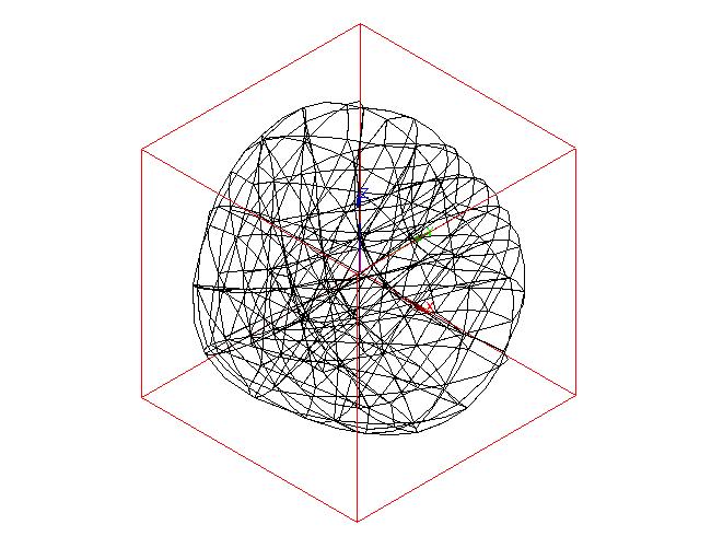
Modal warp ( \(2469.64\mathrm{Hz}\) ) Modal warp ( \(2469.64\mathrm{Hz}\) )
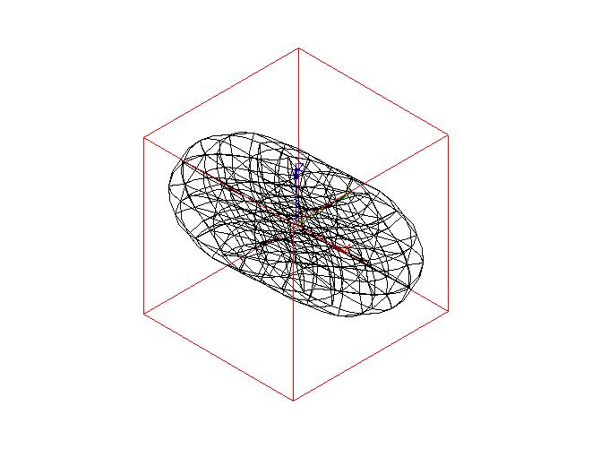
Modal deformed ( \(2470.84\mathrm{Hz}\) )