1. Modeling A

1.1. Problem description

1.1.1. Objective

The objective of this modeling is to determine the first 11 natural frequencies of the embedded beam, in the presence of multiple modes, using the following four methods:

• SORENSEN method,

• LANCZOS method,

• BATHE and WILSON method

• Reverse iteration method

1.1.2. Geometry

1.1.3. Material properties

The material is linear isotropic elastic:

• Young’s module \(E=210000.{10}^{6}N/{m}^{2}\),

• Poisson’s ratio \(\nu =0.3\),

• density \(\rho =7800\mathrm{Kg}/{m}^{3}\)

1.1.4. Boundary conditions and loading

The beam is embedded at point \(A\).

1.2. Characteristics of modeling

1.2.1. Meshing

The wire mesh can be built interactively using Salomé. All you have to do is define the points \(A\), \(B\) and then the line \(\mathrm{AB}\). The size of the elements is the same. In the Salome mesh module, we can declare, based on geometry, point \(A\) as a node group, then \(\mathrm{AB}\) as a group of elements. Then the mesh will be saved in MED format.

Euler’s right beam elements (POU_D_E) will be used for modeling.

The mesh consists of 10 SEG2 and 11 knots.

1.2.2. Aster command file

The main steps of the calculation with*Aster* will be:

Reading the mesh in MED format (LIRE_MAILLAGE (“FORMAT =” MED”)).

Definition of the finite elements used (AFFE_MODELE). The group of elements composing the beam will be assigned modeling POU_D_E.

Material definition and assignment (DEFI_MATERIAU and AFFE_MATERIAU). The mechanical characteristics are identical throughout the structure.

Assigning the characteristics of the beam elements (AFFE_CARA_ELEM). The cross section of all the elements of the beam is the same.

Assigning boundary conditions (AFFE_CHAR_MECA).

Calculation of elementary stiffness matrices (CALC_MATR_ELEM ((OPTION =” RIGI_MECA “)).

Calculation of elementary mass matrices (CALC_MATR_ELEM ((OPTION =” MASS_MECA “)).

Numbering the unknowns of the system of linear equations (NUME_DDL)

Assembly of elementary mass and stiffness matrices (ASSE_MATRICE).

**Note:* to go faster we can use the macro ASSEMBLAGE to build the matrices!

Question #1:

• Calculate the 11 smallest natural frequencies and the first associated modes (CALC_MODES [U4.52.02]).

• Print the proper modes (IMPR_RESU) in MED format for viewing in Salome.

Question #2:

• Calculate the natural frequencies and the first associated modes present in the frequency band \(0\mathrm{Hz}\) and \(6000\mathrm{Hz}\), with the four methods SORENSEN, LANCZOS, BATHE, QZ (CALC_MODES [U4.52.02], keyword factor SOLVEUR_MODAL =_F (METHODE =…)) then by inverse iterations (simple keyword OPTION =” AJUSTE “).

• Print the proper modes (IMPR_RESU) in MED format for viewing in Salome.

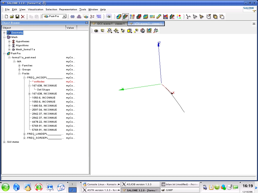
1.3. Help for Post-Treatment under Salome

The different steps for visualizing modal deformations with Salomé are as follows:

Start Salome on Linux

Click on File/Open and select the Salome database (hdf) containing the geometry and the mesh.

Start the Post-Pro post-processing module

Click on File/Import/ MED file and select the file MED containing the specific modes to be viewed

Deploy the Post-Pro line tree completely in the Object Browser in order to see all the movement fields in detail.

Click on one of the fields and with the right mouse button click on Deformed Shape. (the*modal warp is shown).

Deploy the line containing the visualized field, then click on Def. Shape and then click on the right mouse button and select Sweeper to animate the deformation.

1.4. notes

Best practice is to use the “BANDE” option instead of “PLUS_PETITE” or “CENTRE”.

The number of frequencies is determined automatically by the Sturm test and thus all multiplicities are taken into account.

The “SORENSEN” method is the fastest (despite its iterative nature which allows for better precision)

We project onto a smaller space (compared to “TRI_DIAG” and “JACOBI”) and we only do a factorization (compared to the inverse power algorithms implemented when we use OPTION =” AJUSTE “/” SEPARE “/” PROCHE “).

In the presence of multiple modes, the slightest modification of the configuration of the modal method (or of the associated tristraw NUME_DDL…) produces different eigenvectors.

But they always create the same clean space,

To be convinced of this, we can visualize the modal deformations or sum the effective modal masses.

	TRI_DIAG		SORENSEN
	MASS_EFFE_DY	MASS_EFFE_DZ	MASS_EFFE_DY	MASS_EFFE_DZ
Mode 1	3.16920	2.80830	1.13915	4.83834
Mode 2	2.80672	3.17077	4.83834	1.13915
TOTAL	5.97592	5.97907	5.97749	5.97749

1.5. Tested sizes and results

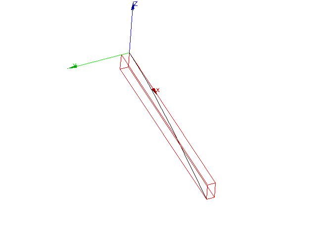
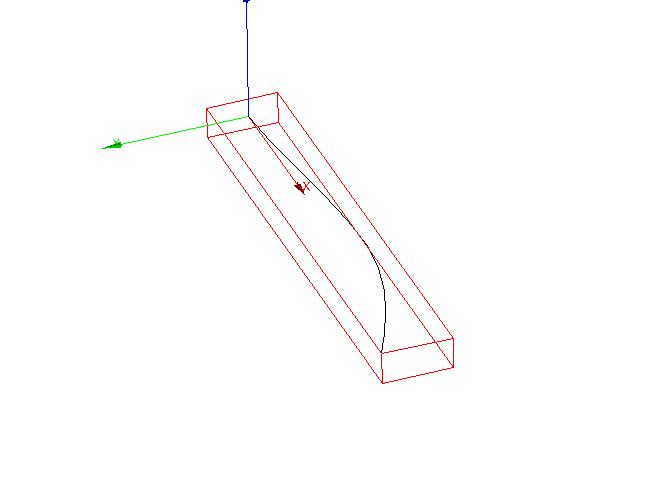
The results obtained with the method of SORENSEN are presented in the table, and in the figures below

Mode	Frequency in \(\mathrm{Hz}\) (Method SORENSEN)
1	1.67638E+02
2	1.67638E+02
3	1.05060E+03
4	1.05060E+03
5	1.48054E+03
6	2.59704E+03
7	2.94237E+03
8	2.94237E+03
9	4.47822E+03
10	5.76991E+03
11	5.76991E+03

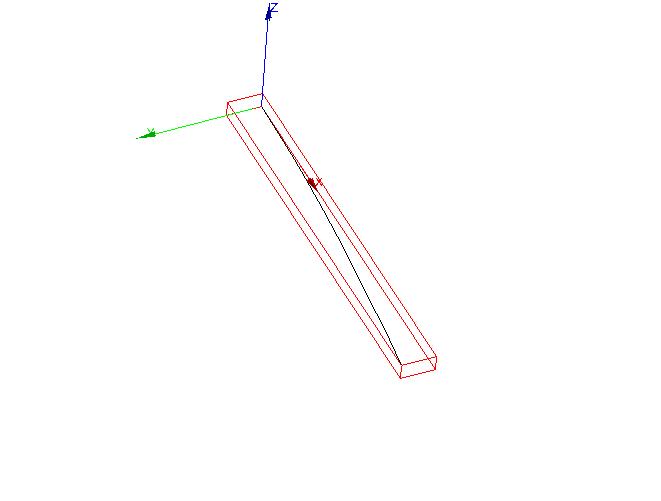
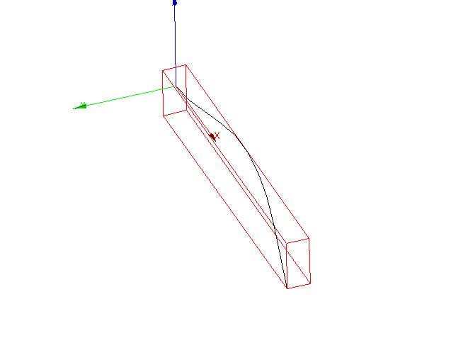
Modal warp ( \(167.638\mathrm{Hz}\) ) Modal warp ( \(167.638\mathrm{Hz}\) )

Modal deformation (:math:`1050.60mathrm{Hz}`) **** (Modal deformation**:math:`1050.60mathrm{Hz}`**) **

Modal deformed ( \(1480.54\mathrm{Hz}\) )