4. B modeling#
4.1. Characteristics of modeling and meshes#
Digital mesh:
The digital mesh is done directly in ASTER format. It has 4 knots and 3 discreet stitches.
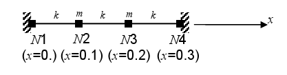
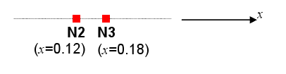
Experimental mesh:
The measurement mesh includes only 2 point elements and 2 nodes:
4.2. Characteristics of the measurements#
The experimental measurements provided are:
At node \(\mathrm{N3}\):
The data are axial displacements, multiplied by \(–1/\sqrt{2}\), and applied in the \(-x\) direction. The local orientation specified in the command file is \((45.0.0.)\)
The time sampling is constant: the initial time is \(0s\), the time step is \({10}^{-3}s\), and the number of moments is 1001 (i.e. up to a final time of \(1s\)).
At node \(\mathrm{N2}\):
The data is the axial displacements, applied in the \(X\) direction.
The time sampling is variable: all the moments are indicated from \(0s\) to \(1s\), in steps of \({10}^{-3}s\) (1001 moments in total).
The values are derived from the analytical calculation carried out with Maple.
4.3. Characteristics of the modal base#
The only two modes are stored in a mode_meca concept, created by the DEFI_BASE_MODALE command. The interface, of the Craig-Bampton type, is placed on the following degree of freedom in movement \(x\) of the node \(\mathrm{N2}\) (corresponding to the mass \(\mathrm{m1}\)). The modal base therefore contains a dynamic mode (with \(\mathrm{N2}\) locked) and a static mode.
4.4. Tested values#
Identification |
Reference |
Aster_code |
difference |
||
at*t* = 0.1 s |
1.745 10—4 |
1.745 10—4 |
0.01% |
||
at*t* = 0.3 s |
6.797 10—4 |
6.797 10—4 |
0.01% |
||
DEPL_X |
At node \(\mathrm{N2}\) |
at*t* = 0.5 s |
—1.217 10—3 |
—1.217 10—3 |
0.01% |
(\(m\)) |
(mass 1) |
at*t* = 0.7 s |
5.214 10—4 |
5.214 10—4 |
— 0.01% |
at*t* = 0.9 s |
9.031 10—4 |
9.031 10—4 |
0.00% |
||
at*t* = 0.1 s |
9.154 10—6 |
9.154 10—6 |
0.00% |
||
at*t* = 0.3 s |
6.414 10—4 |
6.414 10—4 |
0.00% |
||
DEPL_X |
At node \(\mathrm{N3}\) |
at*t* = 0.5 s |
—8.636 10—4 |
—8.636 10—4 |
0.00% |
(\(m\)) |
(mass 2) |
at*t* = 0.7 s |
—1.107 10—4 |
—1.107 10—4 |
0.03% |
at*t* = 0.9 s |
1.633 10—3 |
1.633 10—3 |
0.02% |
||
at*t* = 0.1 s |
4.586 10—3 |
4.616 10—3 |
0.65% |
||
at*t* = 0.3 s |
—7.598 10—3 |
—7.663 10—3 |
0.85% |
||
VITE_X |
At node \(\mathrm{N2}\) |
at*t* = 0.5 s |
—1.581 10—4 |
—8,000 10—5 |
7.81 10—5m/s |
(\(m/s\)) |
(mass 1) |
at*t* = 0.7 s |
9.382 10—3 |
9.354 10—3 |
— 0.30% |
at*t* = 0.9 s |
—7.481 10—3 |
—7.537 10—3 |
0.75% |
||
at*t* = 0.1 s |
4.328 10—4 |
4.405 10—4 |
1.79% |
||
at*t* = 0.3 s |
3.671 10—3 |
3.640 10—3 |
— 0.84% |
||
VITE_X |
At node \(\mathrm{N3}\) |
at*t* = 0.5 s |
—1.539 10—2 |
—1.536 10—2 |
— 0.20% |
(\(m/s\)) |
(mass 2) |
at*t* = 0.7 s |
2.453 10—2 |
2.457 10—2 |
0.15% |
at*t* = 0.9 s |
—1.899 10—2 |
—1.912 10—2 |
0.68% |
||
at*t* = 0.1 s |
6.112 10—2 |
6.100 10—2 |
— 0.20% |
||
at*t* = 0.3 s |
—1.306 10—1 |
—1.300 10—1 |
— 0.46% |
||
ACCE_X |
At node \(\mathrm{N2}\) |
at*t* = 0.5 s |
1.571 10—1 |
1.600 10—1 |
1.85% |
(\(m/{s}^{2}\)) |
(mass 1) |
at*t* = 0.7 s |
—5.657 10—2 |
—5.800 10—2 |
2.53% |
at*t* = 0.9 s |
—1.124 10—1 |
—1.130 10—1 |
0.53% |
||
at*t* = 0.1 s |
1.562 10—2 |
1.618 10—2 |
3.58% |
||
at*t* = 0.3 s |
—6.031 10—2 |
—6.223 10—2 |
3.18% |
||
ACCE_X |
At node \(\mathrm{N3}\) |
at*t* = 0.5 s |
5.102 10—2 |
5.374 10—2 |
5.33% |
(\(m/{s}^{2}\)) |
(mass 2) |
at*t* = 0.7 s |
7.428 10—2 |
7.043 10—2 |
— 5.19% |
at*t* = 0.9 s |
—2.364 10—1 |
—2.263 10—1 |
— 4.28% |
||
Note:
The speed at the node \(\mathrm{N2}\) at instant \(t=0.5s\) being relatively close to zero, the comparison is carried out for this case in absolute value.