3. Modeling A#
3.1. Characteristics of modeling#
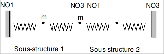
The system is divided into 2 sub-structures:
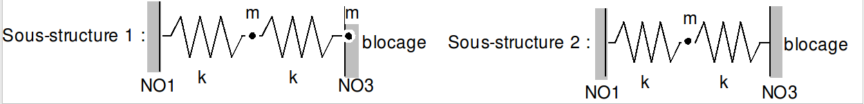
In this situation, the two substructures are connected at the level of the 2nd mass. The dynamic interface of the 1st substructure consists of a mass m at the level of the node \(\mathit{NO3}\) of the mesh and coincides with the dynamic interface of the 2nd substructure which has no mass and is simply blocked at the level of the node \(\mathit{NO1}\).
The eigenmodes of the complete system are calculated using the modal calculation method by substructuring with “Craig-Bampton” interfaces (blocked interfaces). The bases of each substructure are composed of a dynamic mode and a constrained mode.
The transient response of the system is calculated on the modal basis calculated by substructuring.
The time steps used are equal to: \({10}^{-2}s\) in “EULER”, \({10}^{-2}s\) in “”, in “NEWMARK”, \({10}^{-2}s\) in “DEVOGE”, \({10}^{-1}s\) in “ADAPT_ORDRE2” (for the latter, this is the initial time step of the algorithm and the maximum time step is set to formula \(\mathrm{0,15}s\) then formula \(\mathrm{0,2}s\) to optimize calculation time).
3.2. Characteristics of the substructure mesh#
Number of knots: 3
Number of meshes and types: 2 SEG2
3.3. Tested sizes and results#
Calculation by modal recombination without substructuring: Method ADAPT_ORDRE2 and RUNGE_KUTTA_54
Identification |
Reference |
Method: ADAPT_ORDRE2 |
|
Node \({x}_{2}\), displacement (\(m\)) |
4.1700 10—1 |
Knot \({x}_{2}\), speed (\({\mathit{m.s}}^{-1}\)) |
—4.3011 10—1 |
Node \({x}_{2}\), acceleration (\({\mathit{m.s}}^{-2}\)) |
3.3375 10—1 |
Method: RUNGE_KUTTA_54 |
|
Node \({x}_{2}\), displacement (\(m\)) |
4.1700 10—1 |
Knot \({x}_{2}\), speed (\({\mathrm{m.s}}^{-1}\)) |
—4.3011 10—1 |
Node \({x}_{2}\), acceleration (\({\mathrm{m.s}}^{-2}\)) |
3.3375 10—1 |
Calculation by substructuration |
|
Method: EULER |
|
Node \({x}_{2}\), displacement (\(m\)) |
4.1700 10—1 |
Knot \({x}_{2}\), speed (\({\mathrm{m.s}}^{-1}\)) |
—4.3011 10—1 |
Node \({x}_{2}\), acceleration (\({\mathrm{m.s}}^{-2}\)) |
3.3375 10—1 |
Method: DEVOGE |
|
Node \({x}_{2}\), displacement (\(m\)) |
4.1700 10—1 |
Knot \({x}_{2}\), speed (\({\mathrm{m.s}}^{-1}\)) |
—4.3011 10—1 |
Node \({x}_{2}\), acceleration (\({\mathrm{m.s}}^{-2}\)) |
3.3375 10—1 |
Method: NEWMARK |
|
Node \({x}_{2}\), displacement (\(m\)) |
4.1700 10—1 |
Knot \({x}_{2}\), speed (\({\mathit{m.s}}^{-1}\)) |
—4.3011 10—1 |
Node \({x}_{2}\), acceleration (\({\mathit{m.s}}^{-2}\)) |
3.3375 10—1 |
Method: RUNGE_KUTTA_32 |
|
Node \({x}_{2}\), displacement (\(m\)) |
4.1700 10—1 |
Knot \({x}_{2}\), speed (\({\mathit{m.s}}^{-1}\)) |
—4.3011 10—1 |
Node \({x}_{2}\), acceleration (\({\mathit{m.s}}^{-2}\)) |
3.3375 10—1 |
Method: ADAPT_ORDRE2 |
|
Node \({x}_{2}\), displacement (\(m\)) |
4.1700 10—1 |
Knot \({x}_{2}\), speed (\({\mathrm{m.s}}^{-1}\)) |
—4.3011 10—1 |
Node \({x}_{2}\), acceleration (\({\mathrm{m.s}}^{-2}\)) |
3.3375 10—1 |