1. Reference problem#
1.1. Geometry#
Structure \(\mathrm{2D}\) is a unitary square plate (\(\mathit{LX}\mathrm{=}\mathrm{0,1}\), \(\mathit{LY}\mathrm{=}\mathrm{0,1}\)). A « straight » interface divides the domain into 2 sub-domains.
The interface branches off in the vicinity of the center of square \((\mathrm{0,}0.5)\) with an angle \(\theta \mathrm{=}\mathrm{67,5}°\) from the horizontal.
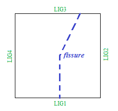
Figure 1.1-1 : Geometry of the cracked plate
The interface is defined analytically by the union of 2 line segments, whose respective equations are:
\(X=0\) for the vertical segment.
\(Y\mathrm{=}2x+0.55\) for the oblique segment.
The intersection point of the 2 line segments is calculated to be located on the edge where the interface forks:
\((\mathrm{0,}0.55)\) for \(A\) and \(B\) models, see
\((\mathrm{0,}0.6)\) for \(C\) and \(D\) models, see
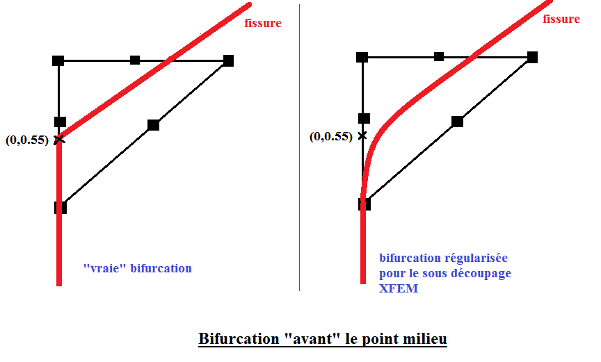
Figure 1.1-2: « zoom » in the vicinity of the bifurcation point
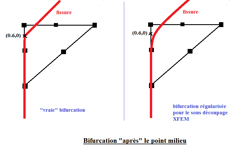
Figure 1.1-3: « zoom » in the vicinity of the bifurcation point
1.2. Material properties#
Young’s module: \(E=210{10}^{9}\mathrm{Pa}\)
Poisson’s ratio: \(\nu =0\)
1.3. Boundary conditions and loads#
Modeling \(A\):
The interface divides the domain into 2 sub-domains. The solution is imposed on the move on each sub-domain, thanks to Dirichlet conditions at the edges:
on edge \(\mathit{LIG2}\): \(\mathit{DX}=-1\) and \(\mathit{DY}=0\)
on edge \(\mathit{LIG4}\): \(\mathit{DX}=\text{+}1\) and \(\mathit{DY}=0\)
There is no contact at the interface level. We are just interested in the movements of the 2 blocks, which can interpenetrate each other.
The imposed Dirichlet conditions also block rigid body movements in the 2 sub-domains.
Models \(B\), \(C\) and \(D\):
Same load as in modeling \(A\).
1.4. Benchmark solution#
Modeling \(A\):
By construction, the field of movement is uniform on each sub-block.
On the sub-domain on the right, we have: \(\mathit{DX}=-1\) and \(\mathit{DY}=0\)
On the sub-domain on the left, we have: \(\mathit{DX}=\text{+}1\) and \(\mathit{DY}=0\)
Modeling \(B\):
Same analytical solution as modeling \(A\)
Modeling \(C\):
Same analytical solution as modeling \(A\)
Modeling \(D\):
Same analytical solution as modeling \(A\)
1.5. Bibliographical references#
GENIAUT S., MASSIN P.: eXtended Finite Element Method, Code_Aster Reference Manual, [R7.02.12]