2. Benchmark solution#
2.1. Calculation method#
The position of the nodes, integration points and integration sub-points is calculated from their coordinates in the local axes of the beam and from the transition matrices between the local axes and the global axes.
By default, local axes and global axes coincide (Figure).
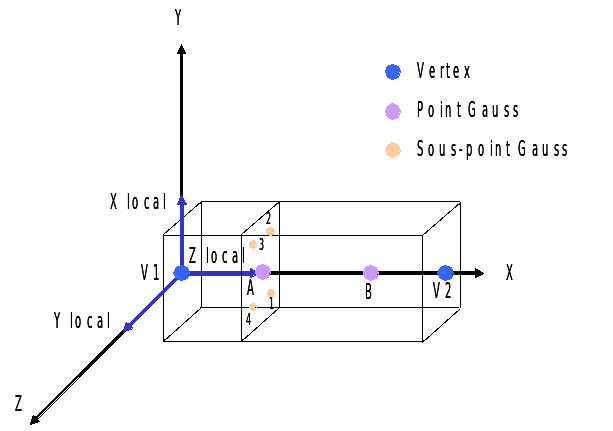
Figure 2.1-a : default position
We apply the two rotations (see Figure) to orient the axis of the beam, and a third rotation to position the straight section:
\(\alpha \mathrm{=}45°\) around \(Z\)
\(\beta \mathrm{=}\mathrm{-}\mathrm{35,26}°\) around the new \(\mathit{Y1}\) axis
\(\gamma \mathrm{=}0°\) or \(90°\) around the new \(\mathit{X2}\) axis
Note:
we use Code_Aster’s nautical angle conventions (see the keyword ORIENTATIONde AFFE_CARA_ELEM)
The rotation around the \(Z\) axis (\(\alpha\)) is based on the following matrix:
\(\mathit{Tz}(\alpha )\mathrm{=}\left[\begin{array}{c}\mathrm{cos}(\alpha )\\ \mathrm{sin}(\alpha )\\ 0\end{array}\begin{array}{c}\mathrm{-}\mathrm{sin}(\alpha )\\ \mathrm{cos}(\alpha )\\ 0\end{array}\begin{array}{c}0\\ 0\\ 1\end{array}\right]\)
The rotation around the new axis \(\mathit{Y1}\) (\(\beta\)) is based on the following matrix:
\(\mathit{Ty1}(\beta )\mathrm{=}\left[\begin{array}{c}\mathrm{cos}(\beta )\\ 0\\ \mathrm{-}\mathrm{sin}(\beta )\end{array}\begin{array}{c}0\\ 1\\ 0\end{array}\begin{array}{c}\mathrm{sin}(\beta )\\ 0\\ \mathrm{cos}(\beta )\end{array}\right]\)
The rotation around the new axis \(\mathit{X2}\) (\(\gamma\)) is based on the following matrix:
\(\mathit{Tx2}(\gamma )\mathrm{=}\left[\begin{array}{c}1\\ 0\\ 0\end{array}\begin{array}{c}0\\ \mathrm{cos}(\gamma )\\ \mathrm{sin}(\gamma )\end{array}\begin{array}{c}0\\ \mathrm{-}\mathrm{sin}(\gamma )\\ \mathrm{cos}(\gamma )\end{array}\right]\)
So, for any point with coordinates \((X,Y,Z)\) before rotations, we can calculate its coordinates \((X\text{'},Y\text{'},Z\text{'})\) after rotations with the following transformation:
\(\left[\begin{array}{c}X\text{'}\\ Y\text{'}\\ Z\text{'}\end{array}\right]\mathrm{=}\left[\mathit{Tx2}(\gamma )\right]\left[\mathit{Tz}(\alpha )\right]\left[\mathit{Ty}(\beta )\right]\left[\begin{array}{c}X\\ Y\\ Z\end{array}\right]\)
2.2. Reference quantities and results#
The position of some integration sub-points in the global coordinate system is calculated knowing their position in the local axes.
With the angles chosen, the digital application gives:
\(\mathit{Ty1}(\beta )\mathrm{=}\left[\begin{array}{c}0.8165\\ 0\\ 0.5774\end{array}\begin{array}{c}0\\ 1\\ 0\end{array}\begin{array}{c}\mathrm{-}0.5774\\ 0\\ 0.8165\end{array}\right]\) \(\mathit{Tz}(\alpha )\mathrm{=}\left[\begin{array}{c}0.7071\\ 0.7071\\ 0\end{array}\begin{array}{c}\mathrm{-}0.7071\\ 0.7071\\ 0\end{array}\begin{array}{c}0\\ 0\\ 1\end{array}\right]\)
and
\(\mathit{Tx2}(\gamma )\mathrm{=}\left[\begin{array}{c}1\\ 0\\ 0\end{array}\begin{array}{c}0\\ 1\\ 0\end{array}\begin{array}{c}0\\ 0\\ 1\end{array}\right]\) or \(\mathit{Tx2}(\gamma )\mathrm{=}\left[\begin{array}{c}1\\ 0\\ 0\end{array}\begin{array}{c}0\\ 0\\ 1\end{array}\begin{array}{c}0\\ \mathrm{-}1\\ 0\end{array}\right]\)
For an element of length \(L\mathrm{=}2\mathrm{\cdot }\sqrt{3}m\), the distance of the second Gauss point from the first node is:
For elements POU_D_EM (models A and B) that have two Gauss points:
\((\frac{1}{2}+\frac{1}{2\sqrt{3}})L=1+\sqrt{3}=2.7320508075688772m\)
For elements POU_D_TGM (models C and D) that have three Gauss points:
\(\frac{L}{2}\mathrm{=}\sqrt{3}\mathrm{=}1.7320508075688772m\)
The section of the \((\mathrm{0,2}m\mathrm{\times }\mathrm{0,1}m)\) beam is discretized into 4 quadrilaterals (Figure).

Figure 2.2-a: position of the sub-points in the section
The position of the sub-points chosen in the initial coordinate system for models A and B (POU_D_EM) is therefore:
Point |
Sub-point |
\(x\) |
|
|
2 |
1 |
2.73205080807568877 |
-0.05 |
-0.025 |
2 |
2 |
2.73205080807568877 |
0.05 |
-0.025 |
2 |
3 |
2.73205080807568877 |
0.05 |
0.025 |
2 |
4 |
2.73205080807568877 |
-0.05 |
0.025 |
And the position of the sub-points chosen in the initial coordinate system for the C and D models (POU_D_TGM) is:
Point |
Sub-point |
\(x\) |
|
|
2 |
1 |
1.73205080807568877 |
-0.05 |
-0.025 |
2 |
2 |
1.73205080807568877 |
0.05 |
-0.025 |
2 |
3 |
1.73205080807568877 |
0.05 |
0.025 |
2 |
4 |
1.73205080807568877 |
-0.05 |
0.025 |
2.3. Uncertainties about the solution#
None, exact solution.