5. C modeling#
5.1. Mechanical results#
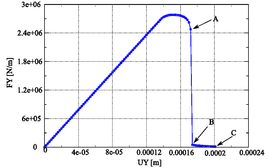
Figure 5.1-1: Force-displacement curve, bi-notched specimen (law MAZARS).
No control method is used. The force-displacement curve obtained is in the. The test piece at time \(C\) is completely broken, with the residual force being close to zero. It is at this moment that the crack opening will be calculated. The pattern of the movements, of the damage and of the equivalent deformation are given in the Figures, and.
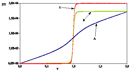
Figure 5.1-2: Movement on the longitudinal axis of the specimen (law MAZARS).
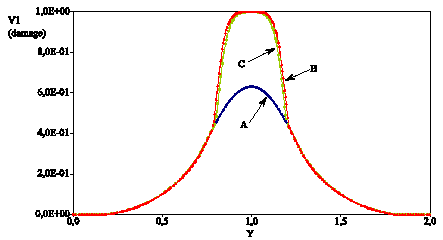
Figure 5.1-3: Damage on the longitudinal axis of the specimen (law MAZARS).
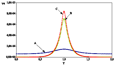
Figure 5.1-4: Equivalent deformation on the longitudinal axis of the specimen (law MAZARS).
5.2. Tested sizes and results#
The crack path found at instant \(C\) is similar to that of.
The quantities tested are the same as in modeling B.
In summary:
Quantity tested |
Test type |
Precision requested |
Test case accuracy |
\(\mathit{DY}\) |
Analytics |
\(0.03m\) |
|
Openness |
Analytics |
:math:`10`% |
:math:`0.683`% |
\(\mathit{DY}\) |
Non-regression |
\(0.01m\) |
|
Openness |
Non-regression |
:math:`1`% |
:math:`0.683`% |
5.3. notes#
The crack path found is more accurate than for modeling B. This is due to the damage law used, which is less localized at the break.